Abstract

Considering ‘Converging to Convergence’ by Kremer, Willis and You (2021), this project investigates absolute/unconditional convergence globally between 1800 and 2020. Beginning with key convergence theories and frameworks, global GDP per capita data from Gapminder.org is used to create percentiles for an analysis of convergence/divergence over time. The data is then logged and evaluated for the geometric mean, the standard deviation (σ-convergence), the coefficient of skewness and excess kurtosis. Through an analysis of these statistics, this project concludes that absolute/unconditional convergence is not present. Overall, divergence is present, with indications of convergence attributed to the growth trajectories of China and India. 

Literature Survey

Keywords: Absolute Convergence, Sigma-convergence

Introduction: Convergence has a long history in economic literature, with theory and framework heavily debated. Recent studies of absolute convergence have applied the theory regionally or to clusters of similar countries, rather than to a global distribution (Ahmad, 2006; Duncan and Fuentes, 2006).[1][2] However, a recent study by Kremer, Willis and You (2021) has brought global absolute convergence back into discussion, with its critics highlighting measurement issues and caveats to drawing broader conclusions about economic growth.

Survey: Dvoroková (2016) reviews the main convergence measurement frameworks, β-convergence and σ-convergence. Denoting the former as a measurement of countries converging to a steady-state and the latter measuring the catch-up effect amongst economies, σ-convergence and panel data are favoured for a more detailed analysis. [3]

Johnson and Papageorgiou (2020) showed that from 182 countries between 1960 and 2010, the recent increase in global wealth was distributed unequally. They concluded that growth in low-income countries is episodic and not in line with a traditional theory of absolute convergence. [4]

Kremer, Willis and You (2021), using varying sources from 1960 to 2017, concluded that global economies have trended towards absolute convergence since the late 1980’s. Through a β-convergence framework, the study argued that this trend is consistent with neoclassical growth models and that the gap between unconditional and conditional convergence is shrinking. [5]

Acemoglu and Molina (2021) using the data from the Kremer, Willis and You (2021) study, refuted the original findings. Their conclusions showed that the use of β-convergence biased the data, arguing that changes in convergence patterns were the result of a statistical artefact common to measurements of this nature. [6]

Conclusion: Initially, this project aims to contribute to the recent debate by using a larger sample size than similar studies (GDP per capita data from 195 countries between 1800 and 2020). Commonly seen in convergence literature, this study stratifies GDP per capita income levels (in the form of percentiles) to provide a base for an analysis of long-run growth patterns. As Kreymer, Willis and You (2021) and studies, such as Barro and Sala-i-Martin (1992) and Mankiw et al. (1992), that typify convergence literature focus on β-convergence, this project uses σ-convergence (in conjunction with summary statistics) to analyse global convergence. [7][8] Some contemporary literature differentiates between absolute/unconditional convergence measurements and its corresponding economic theory, in order to adapt for regional convergence episodes which, ultimately, sit in line with ‘conditional’ or ‘club’ convergence theories (Tiruneh, 2003; Zulfiqar, Chaudhary and Aslam, 2017). [9][10] This project separates the measurement models and theories for clarity when applied to a global distribution. 

Absolute Convergence:

A Contribution to the Current Debate[1]

Introduction

In contemporary convergence literature, a recent study by Kremer, Willis and You (2021) argued that global economies have trended towards ‘absolute convergence’ since the late 1980s, stating that absolute/unconditional convergence, ‘poor countries growing faster than rich, unconditionally’, is present from 2000 to 2015 (Kremer, Willis and You, 2021, p. 2). The paper concluded that the empirical evidence ‘does not support an explanation in which countries catch up only above a certain income threshold’ (Kremer, Willis and You, 2021, p. 27). With seemingly robust figures supporting these claims, critics highlighted the study’s lack of country heterogeneity, ‘a defining feature of the modern growth experience’, which caused challenges and biases when interpretating their estimates (Johnson and Papageorgiou, 2020, p. 132). Acemoglu and Molina (2021) commented that by not properly accounting for fixed differences in nations, the conclusions of the study were largely due to a statistical artifact typical of existing measurement techniques throughout the canon of convergence literature. Considering the above, this paper aims to contribute to the debate by investigating the presence of absolute/unconditional convergence globally from 1800 until 2020 using basic statistical analysis. Beginning with an introduction into the main theories and techniques used to investigate convergence, this project uses the ‘Great Divergence’ as a starting point to examine changes in global income distributions over time (Pomeranz, 2000, p. 1). This is undertaken by arranging GDP per capita data from 195 countries (between 1800 and 2020) into seven percentiles, where the n^th percentile is the income per capita that n% of the global population have less than (see Figure 1). Viewing the distribution in this way allows for a visual analysis of convergence/divergence between sets of nations with similar per capita income. The natural log of the data is then taken and reapplied to the percentiles to give Figure 2. The logged data is then evaluated for σ-convergence (the standard deviation), excess kurtosis, the geometric mean and the coefficient of skewness in each year across the distribution of countries. The test for σ-convergence is used to provide a clear numerical analysis of global convergence/divergence. The remaining descriptive statistics contribute crucial details to the analysis of convergence/divergence (depicted in figures 3, 4, 5 and 6). Finally, GDP per capita is used as the central measurement of a nation’s wealth, thus, regional convergence and in-country income distribution are not considered.

Background

Convergence is a macroeconomic ‘catch-up behaviour’ whereby a country’s income growth, usually measured in GDP per capita, accelerates over a short period of time until it reaches a steady state in line with a richer country (Jones, 2018, p. 54). This implies that all economies could eventually converge and that developing countries can potentially grow more quickly than developed ones. From this, three key theories have emerged in the literature: the absolute/unconditional convergence hypothesis states that ‘countries converge to one another in the long-run independently of their initial conditions’; the theory of conditional convergence suggests that ‘countries that are similar in their structural characteristics (e.g., preferences, technologies, rates of population growth, government policy, etc.) converge to one another in the long-run independently of their initial conditions’; club convergence theory states that ‘countries that are similar in their structural characteristics converge to one another in the long-run if their initial conditions are similar’ (Galor, 1995, p. 1). There are two main frameworks used to measure convergence, β-convergence and σ-convergence. β-convergence is based on a neoclassical theory of growth, which suggests that poorer nations initially show higher growth dynamics, implying they can grow faster than rich countries (Dvoroková, 2016). The measure involves ‘regressing the growth in per capita GDP on its initial level for a given cross-section of countries’ where the result of unconditional/absolute convergence is implied ‘if the coefficient on initial per capita GDP is negative and statistically significant’ (Boyle and McCarthy, 1997, p. 1). Whereas σ-convergence uses a ‘measure of dispersion’ to examine the distribution of ‘income per capita (or worker) across countries’ (Dalgaard and Vastrup, 2001, p. 283). The most frequently used measures of dispersion are the coefficient of variation and the standard deviation of log GDP per capita (Dalgaard and Vastrup, 2001).[2] This project has chosen σ-convergence using the standard deviation of log GDP per capita because of its simplicity in interpretation, its appropriateness for panel data and its lack of biases compared to its β-convergence counterpart (Boyle and McCarthy, 1997; Dvoroková, 2016). In the literature, investigations into convergence are often studied in comparison with the Great Divergence.

The Great Divergence was a socioeconomic shift (beginning at the advent of the industrial revolution in the 19^th century) where the national incomes of nations in Western Europe and the New World began to diverge rapidly away from the global norm, establishing themselves as the dominant nations (Pomeranz, 2000). A variety of explanations have been put forward to explain the sudden change in economic trajectories, ranging from geography to cultural institutions and colonialism. Pomeranz (2000), known for popularising the term, purports that the two main factors responsible for the industrial growth of Northwest Europe were the location of coal and access to trade with the New World. Although explanatory theories differ between schools of economic thought, the Great Divergence has become a staple of convergence literature, often used as a starting point for longitudinal studies of convergence/divergence theories and modelling.

Data

Beginning with Professor Wright’s initial work presented a unique peculiarity, as the ‘raw’ data contained existing manipulations which had to be fully understood before making any further transformations or conclusions. All raw data (including Professor Wright’s work) is sourced from the non-profit organisation Gapminder (Gapminder.org, 2021). Working with the existing data manipulations, this project began by updating version 26 of the Gapminder GDP per capita dataset (in constant price 2011 PPP dollars) to the most recent version of the dataset (version 27), showing figures in constant price 2017 PPP dollars (see Appendix A). The population data originates from Gapminder’s latest Population dataset, version 6, which itself is a composite of three main sources (see Appendix B).

As information from the Maddison Project Database features heavily in these datasets, it is important to note that as a subset, estimates drawn from the historical data will lack some degree of accuracy (Wright, 2022). Similarly, as all the data is based on a composite of sources collated by Gapminder.org, the further inaccuracies inherent to this are recognised as unavoidable measurement problems of longitudinal convergence analysis.

The percentiles used to display figures 1 and 2 are constructed from the formula (Wright, 2022):

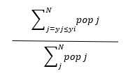
Where ‘N’ is the number of countries, ‘j’ is the total population, ‘yj’ is the GDP per capita income of a given country ‘j’, and ‘yi’ is the GDP per capita income of countries greater than or equal to ‘yj’, in a particular year (see excel sheets ‘pop’ and ‘prank y’). The percentiles rank the countries from lowest to highest GDP per capita income for a given year. Taking this rank as the base for the pertaining population sizes for each country, the formula then takes a given country’s population ‘j’ and divides it by the total global population. This gives a proportion of the global population with a GDP per capita income less than or equal to the selected population of country ‘j’. To construct Figure 1, each line depicts an average percentile which is calculated by finding the average GDP per capita income in a given year of the country just above and just below the desired percentile i.e. the figure for the 5% percentile in the year 2000 is the average of the GDP per capita income for Burkina Faso and Togo (see excel sheet ‘percentiles data’). The calculations for Figure 2 are the above calculations used with the natural log of GDP per capita income. Figures 3, 4, 5 and 6 are measures of the geometric mean, the standard deviation (σ-convergence), coefficient of skewness and excess kurtosis drawn from the natural log of GDP per capita income distributions in all years.

Analysis

The conclusions of this paper breakdown into three parts. The analysis of the percentiles data over time, which did not adequately show absolute/unconditional convergence. An investigation into the convergent results of the 10^th, 30^th and 50^th percentiles, which are explained by the remarkable growth of China and India. The results of the σ-convergence test and the findings from the descriptive statistics, which conclude by presenting a lack of absolute/unconditional convergence in the distribution.

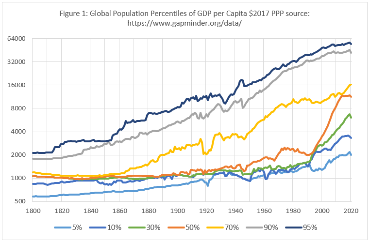
Looking at figures 1 and 2, steady divergence is present throughout the distribution, with a lack of absolute convergence indicated by the difference in growth patterns between the upper and lower percentiles. Primarily, there is markedly strong and stable growth in the 90^th and 95^th percentiles when compared to the inconsistencies of the 5^th, 10^th and 70^th percentiles. This seems to be due to the turbulent nature of growth in the lower percentiles, highlighted by the deceleration of the 70^th percentile in the 1970s and the oscillations of the 5^th and 10^th percentiles. As stated by Johnson and Papageorgiou (2020), growth, especially in developing nations, ‘is highly episodic’ and characterised by periods of accelerations and decelerations ‘often leading to disasters’ (Johnson and Papageorgiou, 2020, pp. 141-144). These turbulent ‘growth spells’ are noted as being less present in ‘advanced economies’, leading to more stable and sustained growth, as depicted by the 90^th and 95^th percentiles in figures 1 and 2 (Johnson and Papageorgiou, 2020, pp. 141-144).

 

Initially, the 10^th, 30^th and 50^th percentiles show the presence of unconditional/absolute convergence from around 1990. However, these anomalous results can be more accurately explained by the growth trajectories of two singular nations in the distribution. The hockey-stick-like catch-up behaviour of the 10^th, 30^th and 50^th percentiles in recent decades can be attributed to the economic growth of China, as it moves from 10^th to 70^th percentile, and India, as it moves from 10^th to 30^th percentile (Wright, 2020). The upturns of these three percentiles are seemingly at the expense of the 70^th percentile, which is relatively flat and falls behind the 90^th and 95^th percentiles as a result (Wright, 2020). These observations emphasise the lack of absolute convergence and highlight only the ‘successful convergence experiences’ of certain nations in ‘South and East Asia’ (Johnson and Papageorgiou, 2020, p. 145). It could be further surmised that the growth trajectories of these nations might partly account for the trends in skewness and excess kurtosis discussed in the proceeding paragraphs. However, when removed from the distribution, the skewness and excess kurtosis results did not significantly change.

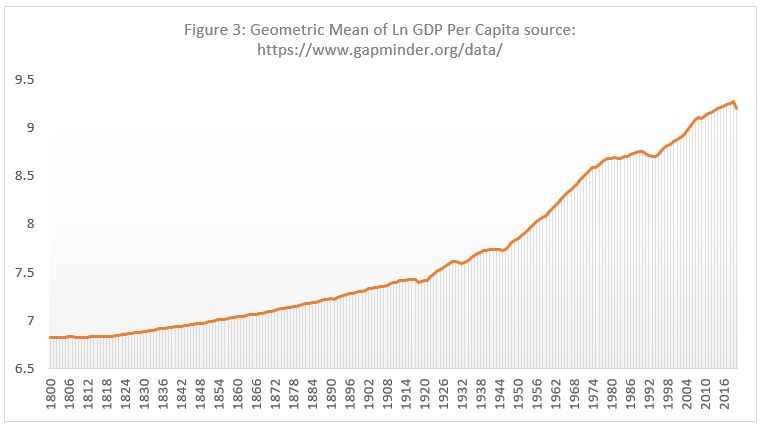
As a base for a final comment on figures 1 and 2, it is important to note the marked increase in global wealth since the start of the 20^th century, indicated by the geo-metric mean of log GDP per capita in Figure 3. Considering this increase, the percentiles data reflects the uneven distribution of this marked global prosperity, highlighted by the starkly stable growth of the 90^th and 95^th percentiles in comparison to the rest of the distribution (particularly the 5^th, 10^th and 70^th percentiles).

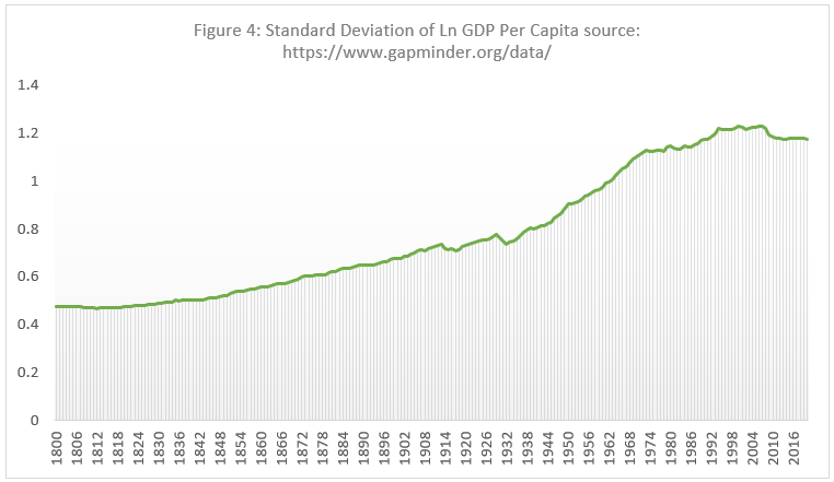
In Figure 4, we can clearly see that a test for σ-convergence shows progressive divergence in global income levels. Particularly, there is a marked increase in the dispersion of log GDP per capita levels across economies between 1932 and 1973, where the standard deviation increases from 0.7 to 1.1 across the global distribution.

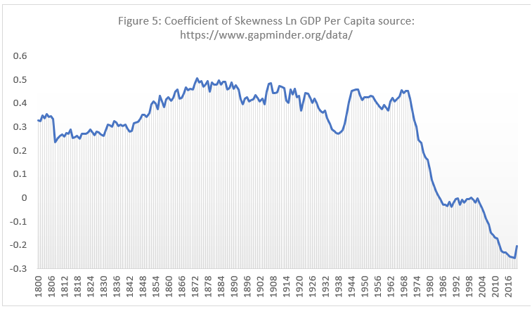
In Figure 5, the coefficient of skewness indicates that the global distribution has not changed markedly between 1800 and 2020, ranging from 0.5 to -0.3. However, there is trend from light negative skewness towards light positive skewness between 1970 and 2019, implying a larger divergence in the richer nations from the mean of the global distribution in recent decades.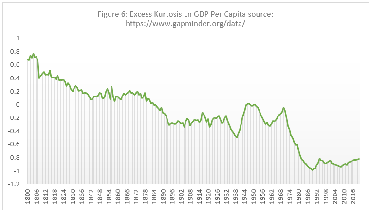

This trend is understood more clearly when considering Figure 6, as the values of excess kurtosis move from 0.7 to -0.8 over the whole period. As there is a flattening of the distribution due to the increasing extreme values in each of the tales, this indicates a progressive divergence between the very richest and very poorest nations over time (with a marked divergence between 1971 and 2020, from -0.04 to -0.8). This finding corresponds to the large gaps (in Figures 1 and 2) between the income levels of the top two percentiles and the 70^th percentile, and between the 70^th percentile and the 5^th to 50^th percentiles. In conclusion, although all nations have become wealthier, the above statistics show that the dispersion of global incomes seemed to have diverged in the long run. Thus, poorer countries have not converged towards richer ones unconditionally.

Conclusion

This project set-out to investigate the presence of absolute convergence globally from 1800 until 2020 using basic statistics. Beginning with the main theories and measurements of convergence, and a brief history of the Great Divergence, this paper gathered GDP per capita data from the non-profit organisation Gapminder for 195 countries (from 1800 to 2020). In conjunction with Professor Stephen Wright, the data was arranged into seven percentiles to allow for a visual analysis of convergence/divergence between sets of nations with similar per capita income. The data was then logged and evaluated for σ-convergence, excess kurtosis, the geometric mean and the coefficient of skewness in each year across the distribution of nations. The evidence from the test for σ-convergence, the summary statistics and the percentiles graphs suggested that divergence was present overall, instead of absolute convergence. Suggestions of absolute convergence in the distribution and percentiles were revealed to be the result of the successful convergence experiences of China and India.

Considering club convergence theories further, accounting for regional convergence would construct a more realistic picture of convergence/divergence patterns globally. Lakner and Milanovic (2015) examined global convergence using a panel database of national household surveys from 1988 to 2008, creating percentiles calculated from the poorest segments of the poorest nations and the richest segments of the richest. Although the percentiles on income data are not directly comparable to GDP per capita data, through discussions with Professor Wright, an initial comparison with this project (using rough estimates to account for the change in GDP constant prices) showed the upper percentiles of national incomes to be remarkably similar, but with illuminating differences in the variety, or ‘clubs’, of nations (Wright, 2022). In contrast to this project’s 95th percentile, the Lakner and Milanovic (2015) study equivalent included the 70th percentile from the USA, Germany’s 80th percentile and the top decile in Brazil and Venezuela. Lakner and Milanovic (2015) attribute this finding to the significant under recording of top incomes globally, which could suggest that the highest deciles of the richest countries are far above the 95th percentiles calculated in both studies. This diversifying of the percentiles regionally is a more accurate depiction of global income movements and any resulting convergence or divergence. This is especially true considering that ‘while country convergence remains monotonically beneficial for poor individuals, its relative importance diminishes as within-country inequality has begun to dominate between-country inequality’ (Pande and Enevoldsen, 2021, p. 3).

 

 

 

 

 

 

 

 

Bibliography

Acemoglu D. and Molina C. A. (2021) ‘Converging To Converge? A Comment’, National Bureau Of Economic Research, NBER Working Paper Series 2021, doi: 10.3386/w28992

Ahmad N. (2006) ‘Corrupt Clubs and the Convergence Hypothesis’ The Pakistan Development Review, 45(4), pp. 1001–1009. Available at: http://www.jstor.org/stable/41260664 [Accessed: 15^th April 2022].

Barro R. J. and Sala-i-Martin X. (1992) ‘Convergence’ Journal of Political Economy, 100(2), pp. 223–251. Available at: http://www.jstor.org/stable/2138606 [Accessed: 15^th April 2022].

Boyle G. E. and McCarthy T. G. (1997) ‘Simple Measures of Convergence in Per Capita GDP: A Note on Some Further International Evidence’, Applied Economics Letters, 6(6), pp. 343-347. Available at: https://core.ac.uk/download/pdf/7050441.pdf [Accessed: 18^th April 2022].

Dalgaard C. and Vastrup J. (2001) ‘On the measurement of σ-convergence’, Economics Letters No. 70(2), pp. 283–287. Available at: https://web2.econ.ku.dk/dalgaard/Work/published/sigma.pdf [Accessed: 18^th April 2022].

Dvoroková K. (2016) ‘Method Matters: Essays on the Selected Econometric Techniques for Modelling of Economic Convergence’, [Conference] International Conference on European Integration, Technical University Of Ostrava, 19^th and 20^th May. Available at: https://is.muni.cz/publication/1372774/VSB_sbornik.pdf [Accessed: 15^th April 2022].

Duncan R. and Fuentes R. (2006) ‘Regional Convergence in Chile: New Tests, Old Results’ Cuadernos de Economía, 43(127), pp. 81–112. Available at: http://www.jstor.org/stable/41954319 [Accessed: 15^th April 2022].

Galor O. (1996) ‘Convergence?: Inferences from Theoretical Models’, The Economic Journal, 106(437), pp. 1056-1069. doi: https://doi.org/10.2307/2235378

Gapminder.org (2022) Gapminder Documentation 001. Available at: https://s3.eu-west-1.amazonaws.com/static.gapminder.org/GapminderMedia/wp-uploads/20210512195520/Documentation_-GDP-per-Capita-v26.pdf [Accessed: 15^th April 2022].

Gapminder.org (2022) Documentation for GDP Per Capita by Purchasing Power Parities for countries and territories. Available at: https://www.gapminder.org/documentation/documentation/gapdoc001_v9.pdf [Accessed: 15^th April 2022].

Gapminder.org (2022) Documentation for Total Population for countries and territories. Available at: https://www.gapminder.org/documentation/documentation/gapdoc003.pdf [Accessed: 15^th April 2022].

Gapminder.org (2022) Population. Available at: https://www.gapminder.org/data/documentation/gd003/ [Accessed: 15^th April 2022].

Gapminder.org (2022) Summary Documentation of V27. Available at: https://www.gapminder.org/data/documentation/gd001/ [Accessed: 15^th April 2022].

Johnson P. and Papageorgiou C. (2020) ‘What Remains of Cross-Country Convergence?’, Journal of Economic Literature, 58(1), pp. 129-175. doi: 10.1257/jel.20181207

Jones C. I. (2018) Macroeconomics. 4^th edn. London: W. W. Norton & Company.

Kremer M. and Willis J. and You Y. (2021) ‘Converging to Convergence’, National Bureau Of Economic Research, NBER Working Paper No. w29484, doi: 10.2139/ssrn.3963712

Lakner C. and Milanovic B. (2015) ‘Global Income Distribution: From the Fall of the Berlin Wall to the Great Recession’, The World Bank Economic Review, Policy Research Working Paper No. 6719, Available at: http://hdl.handle.net/10986/16935 [Accessed: 15^th April 2022].

Mankiw N. G. and Romer D. and Weil D. N. (1992) ‘A Contribution to the Empirics of Economic Growth’ Quarterly Journal of Economics, 107 (2), pp. 407–437. Available at: https://eml.berkeley.edu/~dromer/papers/MRW_QJE1992.pdf?msclkid=80a8ca2dc42711ec81b5b79b6f070a74 [Accessed: 15^th April 2022].

Pande R. and Enevoldsen N. (2021) ‘Discussion of “Converging to Convergence” by Kremer, Willis, and You’, National Bureau Of Economic Research, NBER Working Paper Series 2021, Available at: http://www.nber.org/papers/w28992 [Accessed: 15^th April 2022].

Pomeranz K. (2000) The Great Divergence, China, Europe and the Making of the Modern World Economy. Princeton Classics edn. New Jersey: Princeton University Press.

Quiroga P. A. B. (2007) ‘Theory, History and Evidence of Economic Convergence in Latin America’ Instituto de Estudios Avanzados en Desarrollo (INESAD), 13(1), pp. 6–20. Available at: http://www.jstor.org/stable/resrep00574.4 [Accessed: 15^th April 2022].

Tiruneh M. W. (2003) ‘Absolute Convergence across Time and Space: New Empirical Evidence for an Old Debate’ Ekonomický časopis, 51(10), pp. 1270–1291. Available at: https://www.ceeol.com/search/article-detail?id=93285&msclkid=8cf06d16c42811ec82351d765ec1d9c5 [Accessed: 15^th April 2022].

Wright, Stephen. Professor of Economics. (Personal communication, 8^th February 2022).

Young A. T. and Higgins M. J. and Levy D. (2008) ‘Sigma Convergence versus Beta Convergence: Evidence from U.S. County-Level Data’ Journal of Money, Credit and Banking, 40(5), pp. 1083–1093. Available at: http://www.jstor.org/stable/25096293 [Accessed: 15^th April 2022].

Zulfiqar K. and Chaudhary M. A. and Aslam A. (2017) ‘Convergence Hypothesis: A Cross Country Analysis’ Pakistan Economic and Social Review, 55(1), pp. 229–250. Available at: https://www.jstor.org/stable/26730220 [Accessed: 15^th April 2022].

 

 

 

 

 

 

 

 

 

 

 

Literature Survey References

[1] Ahmad N. (2006) ‘Corrupt Clubs and the Convergence Hypothesis’ The Pakistan Development Review, 45(4), pp. 1001–1009. Available at: http://www.jstor.org/stable/41260664 [Accessed: 15^th April 2022].

[2] Duncan R. and Fuentes R. (2006) ‘Regional Convergence in Chile: New Tests, Old Results’ Cuadernos de Economía, 43(127), pp. 81–112. Available at: http://www.jstor.org/stable/41954319 [Accessed: 15^th April 2022].

[3] Dvoroková K. (2016) ‘Method Matters: Essays on the Selected Econometric Techniques for Modelling of Economic Convergence’, [Conference] International Conference on European Integration, Technical University Of Ostrava, 19^th and 20^th May. Available at: https://is.muni.cz/publication/1372774/VSB_sbornik.pdf [Accessed: 15^th April 2022].

[4] Johnson P. and Papageorgiou C. (2020) ‘What Remains of Cross-Country Convergence?’, Journal of Economic Literature, 58(1), pp. 129-175, doi: 10.1257/jel.20181207

[5] Kremer M. and Willis J. and You Y. (2021) ‘Converging to Convergence’, National Bureau Of Economic Research, NBER Working Paper No. w29484, doi: 10.2139/ssrn.3963712

[6] Acemoglu D. and Molina C. A. (2021) ‘Converging To Converge? A Comment’, National Bureau Of Economic Research, NBER Working Paper Series 2021, doi: 10.3386/w28992

[7] Barro R. J. and Sala-i-Martin X. (1992) ‘Convergence’ Journal of Political Economy, 100(2), pp. 223–251. Available at: http://www.jstor.org/stable/2138606 [Accessed: 15^th April 2022].

[8] Mankiw N. G. and Romer D. and Weil D. N. (1992) ‘A Contribution to the Empirics of Economic Growth’ Quarterly Journal of Economics, 107 (2), pp. 407–437. Available at: https://eml.berkeley.edu/~dromer/papers/MRW_QJE1992.pdf?msclkid=80a8ca2dc42711ec81b5b79b6f070a74 [Accessed: 15^th April 2022].

[9] Tiruneh M. W. (2003) ‘Absolute Convergence across Time and Space: New Empirical Evidence for an Old Debate’ Ekonomický časopis, 51(10), pp. 1270–1291. Available at: https://www.ceeol.com/search/article-detail?id=93285&msclkid=8cf06d16c42811ec82351d765ec1d9c5 [Accessed: 15^th April 2022].

[10] Zulfiqar K. and Chaudhary M. A. and Aslam A. (2017) ‘Convergence Hypothesis: A Cross Country Analysis’ Pakistan Economic and Social Review, 55(1), pp. 229–250. Available at: https://www.jstor.org/stable/26730220 [Accessed: 15^th April 2022].

 

 

 

 

 

 

 

 

Appendix A

According to Gapminder’s official documentation, version 27 of the data has been compiled from 5 main sources: the World Bank, the Maddison Project Database, the IMF, the Penn World Table and version 26. Version 26 of Gapminder’s dataset relies on the first four sources with the addition of surveys and growth rates from UNSTAT, the CIA World Fact Book, Eurostat, various national sources (INSEE, Library of Congress etc.) and Gapminder’s own estimates. The organisation and processing of version 27 is as follows; the years 1990 to 2020 contain data exclusively from the World Bank, published in March 2021 in their World Development Indicators. Using data from version 26 as a base, figures from the 2020 version of the Maddison Project Database are used (where possible, otherwise version 10.0 of the Penn World Table is used) to update historical estimates (adjusted based on the earliest available year). The Maddison Project data was also used for countries with data available from 1820 or earlier without adjustment. In 31 cases, Gapminder version 26 data is used from 1800 to the start of the World Bank data (in 1990) to smooth the ‘discrepancy between estimates’ and to avoid ‘dips or peaks’ in single years. The projections from 2021 up to 2050 are based on IMF forecasts in their World Economic Outlook 2021, April edition. These expected change rates are placed on top of the World Bank estimates. The projection estimates are not used for analysis in this paper.

 

Appendix B

The three main sources are Clio Infra-Population data (version 2015), UN population data from the World Population Prospects 2019 and version 3 of Gapminder’s Population dataset. Version 3’s sources and data break down as follows: from 1950 to projections in 2100, data is taken from the UN’s World Population Prospects 2010 revision, the majority of the historical data from 1800-1949 is drawn from the Maddison Population Dataset, and the following sources are used to fill in gaps in the data: Dr Brian Mitchell’s ‘International Historical Statistics’, the UN Statistics Division, the U.S. Census Bureau, ‘The population of Oceania in the second millennium’ by Caldwell et al (2001), various ‘National sources’, and ‘Undocumented’ ad-hoc sources. Version 6 of Gapminder’s dataset is organised as follows: between 1800 to 1950, the Clio Infra data is used wherever possible, otherwise version 3 of Gapminder’s Population dataset is selected. From 1950 up to 2100, UN population data is used (with forecasts based on the ‘medium fertility variant’). For the years before 1950, small adjustments were made to ‘smooth out the discrepancy between the Clio Infra and UN population data’. Equally, data projections beyond 2021 are not used for this project.