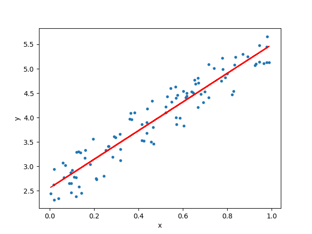
On my journey to learning Python for data analysis, I began by trying to apply everything I had learnt during my Applied Economics Graduate Diploma. More specifically, I wanted to learn how to code out a linear regression. This lead me to a number of different online resources, all claiming to have ‘the best Python code’ to perform a linear regression. However, as everyone knows, it can be hard to find accurate resources online. So, I decided to do a little comparison. 

Now, one thing I could trust was Excel and the statistical formulas I’d learnt from my exams. So, I decided to do a simple linear regression by hand in Excel, to act as a base, in order to compare the coding examples from different websites.    

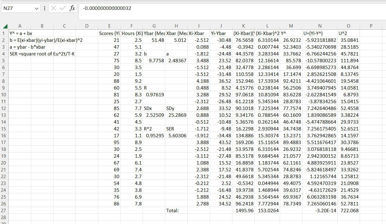
The information above shows 25 data points for ‘Hours’ studied for the X value and the resulting ‘Scores’ on the final exam for the Y value. Performing a linear regression would aim to predict how many hours a student needed to study to gain a certain score on this final exam (based on this sample). 

Just to be clear on notation (and if anyone wants to check my work), the shorthand above should be read as follows: 

Y^ = Y-hat or Predicted Y, Ŷ

E = Sigma, the summation sign, ∑

* = multiply sign in Excel

R^2 = R²

U^2 = U²

U = Residual 

a = Intercept coefficient 

b = X coefficient

^2 = ², squared

xbar = x̄, mean of Xi observations

ybar = Ȳ, mean of Yi observations

SD = Standard Deviation

Bivariate Regression

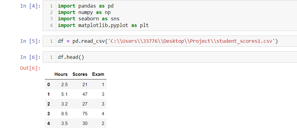
Now I had my base, it was time to test out some code in a Jupyter notebook. I started by importing the libraries I was familiar with and taking a look at the data.

*The data below has an extra column, ‘Exam’, which I added to try out some multiple regression code later on.

I then did a quick bit of exploratory data analysis (I was familiar with this data set, so I didn’t do anything too rigorous).

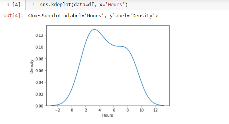
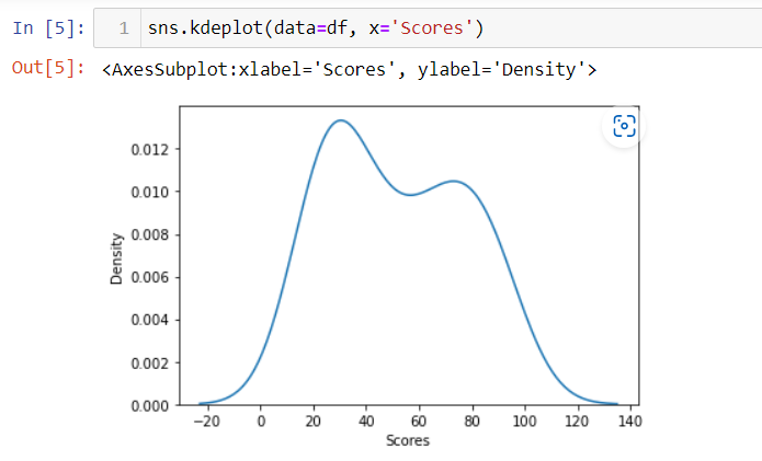
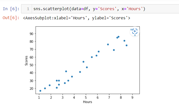
The data seemed positively correlated – that is to say that there seemed to be a linear relationship between the variables and there are no outliers (linear regression models are sensitive to outlier effects). Their distributions were both skewed and slightly abnormal, which at lest gave me some context. Although it’s not the best data to be performing a regression on, my mission was to figure out the best python methods.

Method 1: Sklearn

Relatively simple and easy, I used a method I had learnt from Towards Data Science.com.

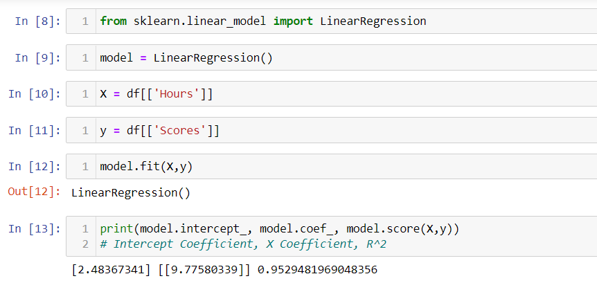
So, after checking my coefficients and R² values with my Excel work, I could see this method had given me the correct results. 

But, it was also not that useful. I needed something that gave me a readout with more informative statistics (hopefully resembling Stata, which I had used during my studies). So, after looking through various sources, TowardsDataScience.com, W3Schools and more, I stumbled upon Statology.org. Clear, intuitive and detailed, it seemed to be exactly what I needed.

Method 2: StatsModels

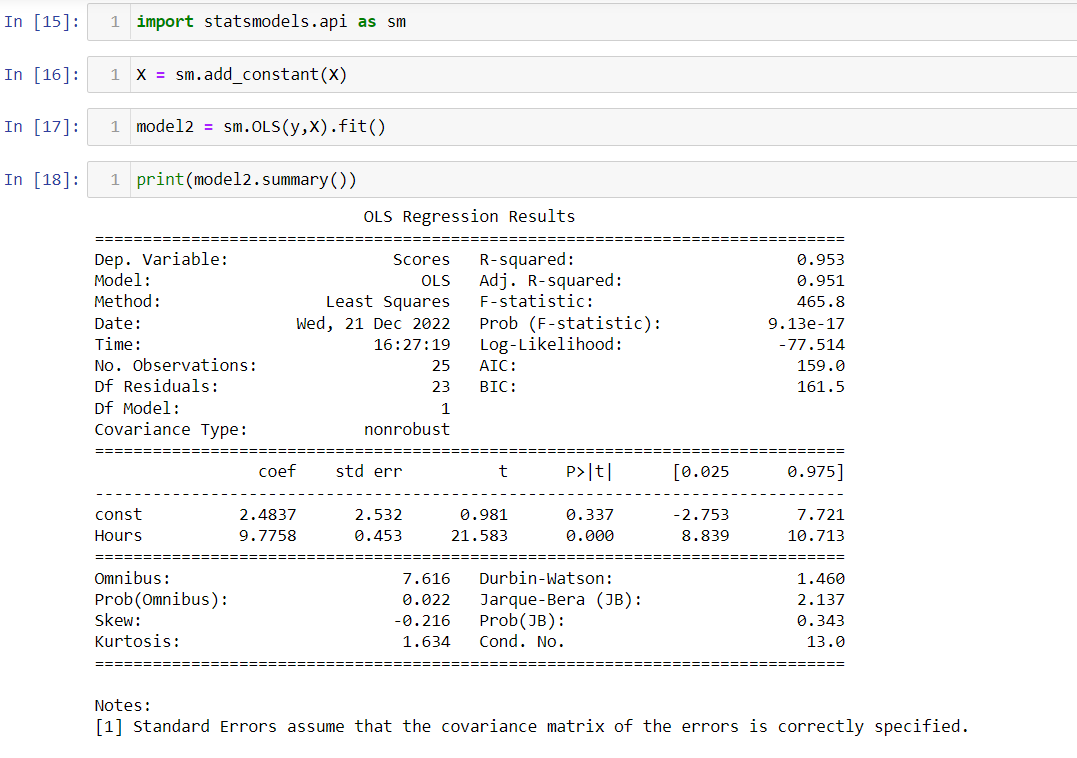
I began by importing the ‘statsmodels’ library, calling the OLS model function (which required me to add an intercept value as it’s not included) and then printed out this very helpful summary. 

Firstly, it all matched with the Excel base work and the former Python code. But, as you can see, it had even more useful information, such as the R-squared value (the measurement of how much of the independent variable is explained by changes in our dependent variable), the Adjusted R-squared value (used to compare the goodness-of-fit for regression models that contain differing numbers of independent variables, but the same dependent variable), the P-values for my coefficients (for determining the significance of the coefficients), the F-statistic (which tells you if a group of variables are jointly significant) and its P-value and some Test Statistics. Secondly, it appears that my X variable was useful in explaining the variation in my Y variable, although my R-squared value was clearly a bit high. Looking through Statology.org further, I realised that I had  found a repository for Python code for statistical testing.

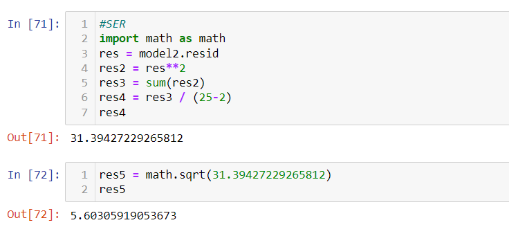
*Except for the SER, Standard Error of Regression, which I couldn’t find anywhere online. So, I had to do some quick (and not very elegant) calculations to see if it matched with my Excel work. 

It did.

Standard Error of Regression

Statistical Testing

Following one of the Statology.org guides, I then started testing out and comparing code that measured how robust my simple model was. 

1. Homoscedasticity

Homoscedasticity is a situation where the error term (sometimes called the “noise” or random disturbance in the relationship between the X and Y variables) is the same across all values of the independent variables. This is very important for having unbiased standard errors and creating confidence intervals. If you want to learn more about homoscedasticity, try Homoscedasticity – Statistics Solutions and Homoscedasticity / Homogeneity of Variance/ Assumption of Equal Variance – Statistics How To.

My first test was to confirm homoscedasticity with a ‘Residual vs Fitted Values’ plot (indicated below by the top right panel). The residuals needed to be randomly scattered around 0 to indicate homoscedasticity.

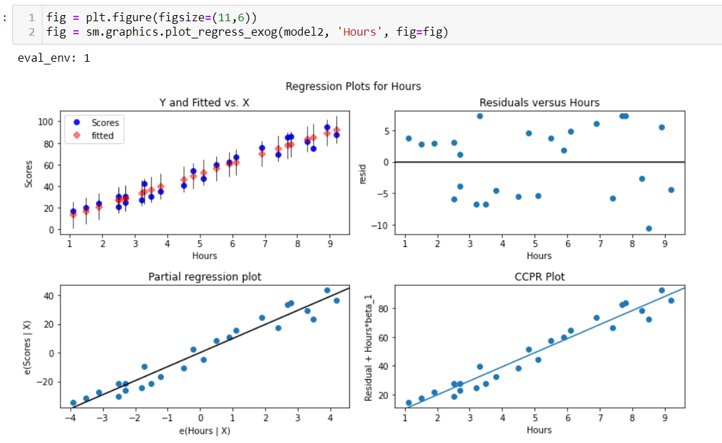
They looked pretty random to me, but I wanted to confirm that with a Breusch Pagan Test (another Statology.org recommendation), where the null states that homoscedasticity is present. Thus, if the p-value was more than 0.05, homoscedasticity was present, and we would’ve failed to reject the null.

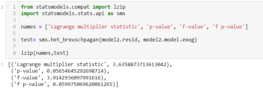
Looks like I was in the clear for that test, just. 

2. Normal Distribution of Residuals

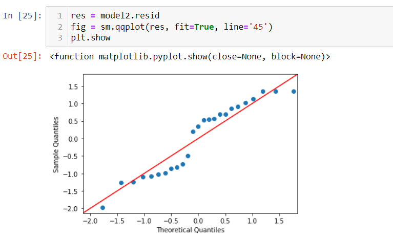
I then wanted to determine if the residuals were normally distributed with a QQ Plot and a Jarque-Bera test using ‘scipy’. 

According to Statology.org, the QQ Plot’s data should roughly follow the line to indicate normality. In the case of the Jarque-Bera test, I knew that it should always gives a positive number and the further away that number was from 0, the more the data did not follow a normal distribution. Equally, if the P-value was greater than 0.05, it would fail to reject the null, meaning that the data would not be significantly different from a normal distribution. 

QQ Plot

Jarque-Bera Test

The Jarque-Bera results matched the summary and, based on the two tests, my residuals were normally distributed. 

3. Independence of Residuals

 Next, I wanted to try a Durbin-Watson test to check the independence of my residuals and then compare it with the summary. When residuals are independent, it means that there is no correlation between consecutive residuals and the model is correctly specified. 

Durbin-Watson Test

Now, the value should be between 1.5 and 2.5, ideally 2 (and is usually used for multivariate linear regressions). Close to 0 indicates positive serial correlation. Closer to 4 means negative serial correlation. The above result suggested that my model had very light positive serial correlation.

Multivariate Regression

 With some solid Python code confirmed, I wanted to apply my findings to a multiple regression model.

The below regression summary came from two X variables, ‘Scores’ and ‘Exam’, the new variable was the data showing the number of practice exams each student took before the final exam.

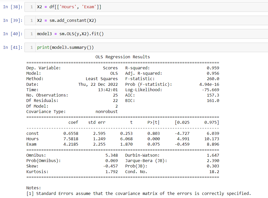
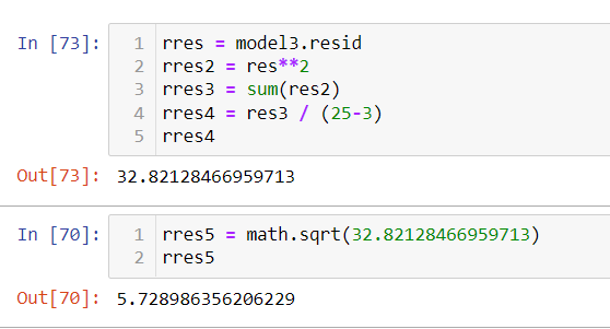
As we can see, the adjusted R-squared was only slightly higher, as was the SER. However, the ‘Exam’ coefficient was now not statistically significant.

This was a good opportunity to try out one more test on the model (suggested, again, by Statology.org). 

Known as the VIF value, or variance inflation factor, it checks for multicollinearity. This is where two or more explanatory variables are highly correlated with each other. As a result, they do not show independent information in the regression model, which then leads to the standard errors of the coefficients being inflated and reduces the accuracy of the p-values. 

According to Statology.org, the VIF score started at 1, meaning no correlation between the X variables. A score between 1-5 meant there was moderate correlation. A score >5 meant there was severe correlation between the x variables.

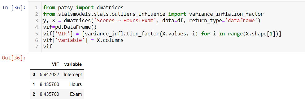
According to this test, my variables were now highly correlated in the model. So, if this was a real model, I would’ve need to consider how my inferences, forecasts and predictions could be drawn from it. Although this would lead to problems interpreting coefficients and p-values, it would not necessarily cause problems for predictions (highlighted by the minor changes in the R-squared and adjusted R-squared values).

Mission accomplished, I successfully used Python to recreate a large part of the linear regression knowledge that I learned on my Applied Economics course.