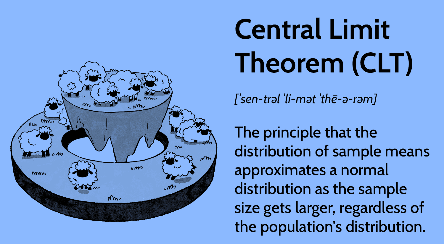
Title:
Statistics Review Part 1
Objective:
The objective of this post was to create a kind of summary document of all the most important ideas, formulas and practices that I’d learnt on my (Applied) Economics Graduate Diploma.
Methods:
Probability Theory, Binomial and Normal Distributions, the Central Limit Theorem
Probability Theory
* Many of the examples and the basis for my explanations are drawn from the seminal text ‘Statistics for Economics, Accounting and Business Studies’ by Michael Barrow, if you want to learn statistics clearly and quickly, I recommend buying this book. My review piece here is an exercise in consolidating knowledge and helping others refresh their stats in general. The image used above is not owned by me and comes from the great online resource Investopedia.com.
The science of probability underlies the theory of statistical inference. In order to draw insights from the population via a sample, we must have a firm understanding of probability and the schools of thought that surround it.
The Frequentist and The Subjective View
Using the toss (or trial) of a (fair) coin as an example, the frequentist view of the probability of heads is equal to the proportion of heads obtained as the number of tosses approaches infinity. The subjective view considers probability to be a degree of belief (that is ‘rational’), with prior beliefs that updated by evidence to form posterior beliefs (this view makes up the basis of Bayesian statistics).
Terms and Formulas
Experiment: an activity, like flipping a coin, which has an outcome.
Trial: a single run of the experiment with the outcome.
Mutually Exclusive: when the outcome of an experiment rules out another, like flipping a coin, you cannot have get both heads and tails.
Event: a collection of outcomes that are being sampled. For example, the probability of rolling odd numbers during one roll of a die – the probability of this event is P(1) = 0.167 + P(3) = 0.167 + P(5) = 0.167 = 0.5.
Compound Events: the probability of event A and event B happening together.
The probability of a single outcome must lie between 0 and 1. The sum of all outcomes’ probabilities during an experiment must sum to 1 – like a coin toss, P(Heads) = 0.5 + P(Tails) = 0.5 = 1.
The OR/Addition Rule is the probability of event A or event B happening, minus the the probability of A and B happening (when the events are are not mutually exclusive) : P(A∪B) = P(A) + P(B) – P(A∩B).
The And/Multiplication Rule is the probability of event A and event B providing the events are independent i.e. one of the events does not conditionally affect the other: P(A∩B) = P(A) x P(B). If they are not independent, but are mutually exclusive P(A∩B) = 0.
If they are not independent but conditional, then the probability of event A and B happening is P(A∩B) = P(A) x P(B|A). The concept of independence is important in statistics as it allows us to analyse an independent variable’s behaviour without worrying about another. Conditional probabilities can be written as P(B|A) – or vice versa – and are read as what is the probability of B given that A has happened. This gives rise to an important part of statistics, Bayes’ Theorem.
Bayes' Theorem
Now, Bayes’ Theorem is a factual statement about probabilities, which we are going to see. The use and interpretation of the result of the theorem is where the controversy lies (something that I will cover in more detail in another article). For now…
P(A|B)= P(B|A) x P(A) / P(B)
…is all you need to know.
Now, let’s put all these formulas to use in a probability table and make everything really simple.
Looking at the probability of a test for a disease working, we want to know the probability that someone has the disease given that they tests positive P(D|TP) and the probability that someone has the disease given that they test negative P(D|TN)? You know these probabilities already:
The probability of having the disease, P(D) = 0.8
The probability of not having the disease, P(ND) = 0.2
The probability of testing positive given that you have the disease, P(TP|D) = 0.7
The probability of testing negative given that you don’t have the disease, P(TN|ND) = 0.95
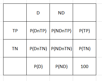
Start here and then use the above formulas to work out the boxes.
Which then gives you this:
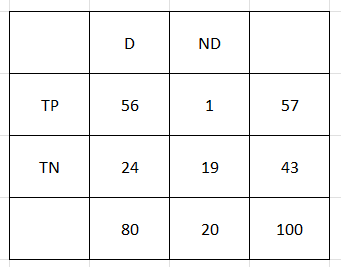
So, P(D|TP) = 56/57 = 98%
and P(D|TN) = 24/43 = 56%
A Probability Distribution
Let’s begin with probability distributions and random variables.
A random variable is like the outcome from the toss of a (fair) coin; it is influenced by chance, it is unpredictable and unknowable, but the range of possible outcomes and their associated probabilities are knowable e.g. P(Heads) = 0.5 , P(Tails) = 0.5.
Using a ‘probability distribution’, it is possible to summarise a random variable by listing (and visualising on a graph) all the possible outcomes of a probability experiment and the probabilities associated with each one i.e. all the values the random variable can take and the probability that each will occur. For example, the number of Heads in 250 tosses of a fair coin is a random variable, which can take a value between 0 and 250. Intuitively, we expect that number to to be around 125, which we can express and check mathematically using the Expected Value, EV(X) = 125.
Probability distributions also tell us something useful about drawing conclusions from a Sample or Population. Take a sample of 10 men in France and find their average height, this would be a random variable. Take all the men of France and find their average height, this would not be a random variable. Why? Well, through the process of taking a sample, it introduces the variability that makes the resulting average a random variable. If you repeated the experiment with another 10 men, the sample mean (our random variable) would be different (slightly). With all the men in France, the mean of the population would not change if we repeated the experiment (assuming the population isn’t constantly changing). In statistics, it is legitimate to make probability statements about random variables, but not parameters.
Binomial Distributions
One of the simplest distributions that a random variable can take is the Binomial. Members of this family of distributions are distinguished by the number of trials, the probability of the outcome occurring and that the probability won’t change between trials. They arise whenever the underlying probability experiment has just two possible outcomes (like a coin flip). Using coins as an example to calculate r = ‘successes/heads’ in n = ‘trials/tosses’, we can use a simple formula to calculate a number of heads in a set of tosses, including their orderings.
* ^r = to the power of ‘r’
* nCr = n!/r!(n-r)!
P(r)=nCr x P^r x (1-P)^n-r
So, for 3 heads in 5 trials, we have: P(r=5) = 5C3 x 0.5³ x 0.5² = 10/32, the probability of 3 heads in 5 tosses in all orderings. With these two parameters n and P, and a random variable r, we can use the shorthand (for the above equation): r~B(n,P). You can also calculate the mean and the variance of a Binomial distribution respectively with these parameters: nP and nP(1-P).
The Normal (Gaussian) Distribution
In the case of a continuous random variable, the Binomial distribution will not suffice. However, we can use the Normal distribution (another family of distributions) instead. Arising usually when a random variable is the result of many random and independent influences (which do not dominate each other), the Normal distribution is characterised by being unimodal (having a single central peak), symmetric, bell-shaped and extends continuously over all the values of X. Its parameters are μ (the mean) and σ (the standard deviation), where the effect of varying σ is to narrow (small σ) or widen (large σ) the distribution. The shorthand can be written as x~N(μ,σ²).
As there are an infinite number of Normal distributions and corresponding tables (one for every value of μ and σ²) we normalise the data and use the Standard Normal Distribution, with a mean = 0 and a variance = 1. This transformation is done via the z score: z = (x – μ)/σ.
For example, let’s take French men’s heights, using the whole ‘population’. It is normally distributed and looks like this x~N(174,92.6), where μ = 174cm and σ = 9.6cm. The question we need to answer is what proportion of men are over 180cm? So, on a graph, what is the area under the Normal distribution to the right of x=180. Using the z score:
z = (180-174)/ 9.6 = 0.63
Firstly, this shows that 180 is 0.63 standard deviations above the mean of the distribution. Using a standard normal table, the value 0.63 corresponds to 0.2643. So, 26.43% of the distribution lies to the right of 0.63 standard deviations above the mean. Thus, in this population, 26.43% of French men are over 180cm. Using this process, you can work out any area under the normal distribution.
The Distribution Of The Sample Mean
One of the most important distinctions in statistical inference is the population vs the sample, it changes many calculations and forms the practical basis for many important theorems. Often, we use the mean of a random sample to make important inferences about the associated population. As the sample mean is a random variable, it also has an associated probability distribution known as the sampling distribution. In statistics, the sample mean, x̄, gives rise to a number of important theorems (including one of the most essential, the Central Limit Theorem):
1. x̄ is normally distributed: any linear combination of independent, Normally distributed random variables is itself Normally distributed. That is to say, the mean, x̄ of a random sample drawn from a population which has a Normal distribution with a mean μ and variance σ², has a sampling distribution which is Normal, with mean μ and variance σ²/n, where n is the sample size.
This first idea is actually quite intuitive, if the population of French men’s heights is a Normally distributed random variable with μ = 174cm and σ² = 92.16, then we would expect that a random sample of 10 men to have a mean/average height around 174cm. The larger the size of the sample, the closer the sample mean would tend to 174cm. In short, the larger the sample size, the closer the sample mean is likely to be to the true population mean.
The shorthand for the Normally distributed sample mean is:
x̄ ~ N(μ, σ²/n)
This can be easily illustrated with an example. Let’s take the random sample of 10 men and workout the probability of them having a mean height greater than 180cm. So, x ~ N(μ, σ²/n), or x ~ N(174, 92.16/10). With a slightly different z score calculation involving the standard error, √σ²/n , this becomes z = x̄ – μ / √(σ²/n) = 180 – 174 / √(92.16/10) = 6/3.04 = 1.98. This means that our sample mean is about 1.98 standard deviations away from the population mean. The value of 1.98 on the standard normal table is an area of 0.0239 in the right-hand tail of the Normal distribution. So, 2.39% of sample means will be greater than or equal to 180cm when the sample size is 10. So, the probability of a random sample of 10 men having a mean height greater than 180cm is 2.39%.
Now, let’s consider what happens when we draw a sample from a non-Normal distribution: enter the Central Limit Theorem.
2. The Central Limit Theorem states that the mean of a random sample, x̄, drawn from a population with mean μ and variance σ², has a sampling distribution which approaches a Normal distribution with mean μ and variance σ²/n, as the sample size approaches infinity.
Turning infinite to finite and Normal to approximately Normal, all that’s left is to know how big of a sample is needed to practically analyse a sample: over 25, in economics, we use 28 – 30 as the lower limit. If the population distribution is particularly skewed, go for more than 30.
Let’s take an example with height again and 50 French men. What is the probability of the sample mean lying within 2.66cm of the true population mean (Figure A: 176.66cm and Figure B: 171.34cm)? By symmetry, Figure A and B must be the same, so let’s workout B, Z = 176.66-174 / √(92.16/50) = 1.96. This makes B=0.475, or 47.5%. This cuts off 2.5% in the upper righthand tail of the distribution. With A being the inverse, this makes up 95% of the distribution. So the probability of the sample mean falling in the range is 95%. This is an important interval known as the 95% probability interval. This interval leads onto estimation and the 95% confidence interval – covered in the next review.