Title:
Statistics Review Part 2
Objective:
The objective of this post was to create a kind of summary document of all the most important ideas, formulas and practices that I’d learnt on my (Applied) Economics Graduate Diploma.
Methods:
Estimation, Confidence Intervals, Hypothesis Testing, Mean Square Error
Estimation
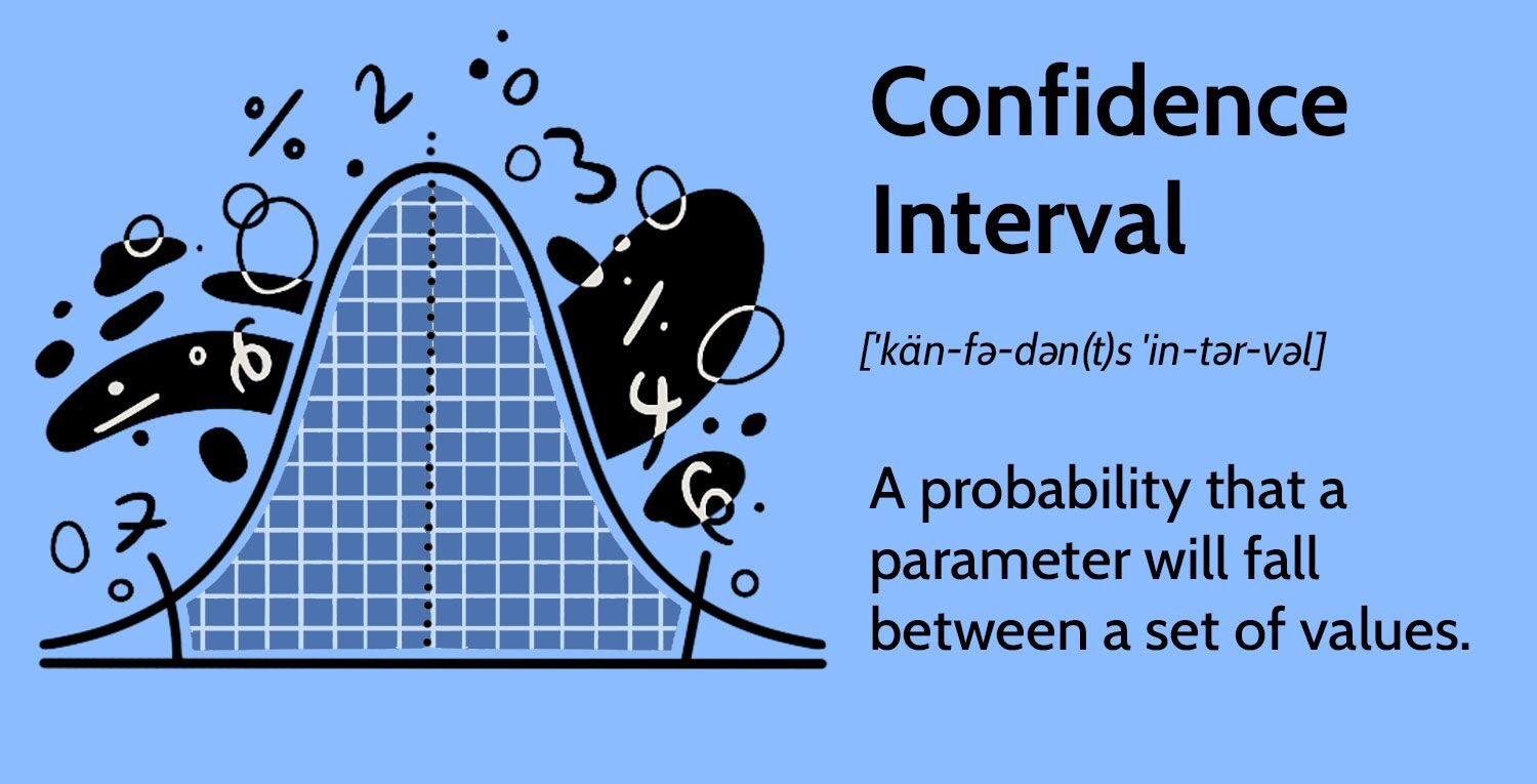
* Many of the examples and the basis for my explanations are drawn from the seminal text ‘Statistics for Economics, Accounting and Business Studies’ by Michael Barrow, if you want to learn statistics clearly and quickly, I recommend buying this book. My review piece here is an exercise in consolidating knowledge and helping others refresh their stats in general. The image used above is not owned by me and comes from the great online resource Investopedia.com.
In the practice of statistics, the sample vales x̄ and s² are often known and not the population parameters μ and σ². So, it’s necessary to ask, given the sample values, what can actually be said about the population?
That’s where estimation comes into play. In economics, we often use the x̄, the sample mean, as a precise, unbiased estimator to make conclusions about the population. But, what exactly does that mean? Well, an estimator that gives the correct on answer on average is considered to be ‘unbiased’ (it’s the best we can hope for really because it’s impossible to check your estimator against the population in practice). Formally, an estimator is unbiased if its Expected Value is equal to the parameter being estimated, which the sample mean is. Now, I’m not going to go through the mathematical proof for that, although during my economics course I did extensively. If you want to, I’m sure you can find it in a suitable textbook or online.
Now for ‘precision’. A precise estimator will tend to give similar estimates for all possible samples and it is usually defined in terms of the variance. The smaller the variance the more precise the estimator. The variance of the sample mean is σ²/n, which explains why larger sample sizes yield on average closer figures to the population (>25).
Mean Square Error
Bias and precision can be combined together into one metric: the mean squared error. It can be defined as equal to the variance + bias². The larger the value of the MSE, the further the estimate is likely to be from the true value, thus the poorer the estimator. The MSE is a metric regularly used in data science to compare different regression models. It should also be noted that a bias estimator is not necessarily an imprecise one – sometimes biasing your results and finding the approximate bias between data may yield a more precise result.
95% Confidence Interval
When using the sample mean (with a sample >25) to gain an estimate of μ (or point estimate to be more exact), we cannot be absolutely sure that it is the same as the population value, μ. So, we need to have some idea of the uncertainty of the estimate. Drawing on the 95% probability from the previous review, we can create an interval estimate known as the 95% confidence interval (yielding 2 values), which indicates that μ lies within 1.96 standard errors of our estimate x̄.
x̄ ± 1.96 √s2/n
A confidence interval is wider, the smaller sample size and the greater the standard deviation. There are a variety of confidence intervals formed with a more general formula (100-a%) to find the z score that cuts off the corresponding amounts in the tails of the standard Normal Distribution – where za is the z score which cuts off the extreme a% (in both tails, hence a/2 in each tail) of the standard Normal Distribution.
x̄ ± za √s2/n
To put this another way, when the σ² variance is known, you can construct a confidence interval as:
x̄ ± za σ/√n
Or, if the sample variance s2 is only known (and the sample size is >25), you can construct a confidence interval as:
x̄ ± za s/√n
BUT, only because of the CLT, meaning that if the population follows a normal distribution, so will x̄, and even if the population is not normally distributed, x̄ is approximately normal in samples >25 i.e.
x̄ – μ / (√σ²/n) ~ N(0,1)
and
x̄ – μ / (√s2/n) ~ N(0,1)
However, for small sample sizes <25 , the last equation above is no longer true, and a t-distribution is necessary.
t-Distributions and Confidence Intervals
Assuming that the parent population is normally distributed, estimating the 95% confidence interval now involves using a t-distribution. Almost identical to the standard Normal distribution, the t-distribution has a larger variance and only has one parameter: the ‘DOF’ Degrees of Freedom, given by the sample size minus 1.
x̄ – μ / (√s2/n) ~ tn-1
Just to be clear, the conditions of use are the sample size being small/<25 and the sample variance is used to estimate the population variance.
Significance and Hypothesis Testing
From estimating the 95% confidence interval, we can also create a formula for hypothesis testing. The process of estimation is appropriate for measurement, whereas hypothesis testing is used for decision-making. To create a hypothesis test, we have the null, depicted by H0 and the alternative H1. Initially, the null is considered true and this presumption is then tested by the sample data.
With a hypothesis, you can make two types of errors: Type 1 – rejecting the null when it is true, and Type 2 – not rejecting the null when it’s false. To test a hypothesis, we use a z score –
Z = x̄ – μ / √s2/n
– coupled with a significance level a = 5% (where 5% is cut off from one side of the Normal distribution for a one-tail test, or 2.5% on both sides for a two-tail test) to give us a critical value. For a one-tailed test at a significance level of 5%, the critical value is 1.64 and for a two-tailed test, it is 1.96. One-tailed tests are concerned with alternative hypotheses that are below or above a specific value:
H0: µ = 5000
H1: µ < 5000
Or
H0: µ = 5000
H1: µ > 5000
In a two-tailed test, the hypothesis test is concerned with a statement:
H0: µ = 5000
H1: µ ≠ 5000
Let’s look at some examples to make this clear. First, a one-tailed test. A sample of 100 factory workers found that the average overtime worked in the previous month was 7.8 hours with a standard deviation of 4.1 hours. Test the hypothesis that the average for all/the population of workers is 5 hours or less at a = 5%. The critical value here 1.64.
H0: µ = 5
H1: µ > 5
Z = (7.8 – 5)/( √(4.12/100)) = 6.8
As 6.8 > 1.64, we reject the null in favour of the alternative hypothesis with 95% confidence: the average for the population of workers is greater than 5 hours.
Next, a two-tailed test. An investor wants to buy a franchise and needs to check the claim that the average business makes on average £5000. From a sample of 26 stores, the mean is £4900 and the standard deviation is £280, test the hypothesis that the average store in the franchise makes £5000.
As we are concerned with values above and below £5000, we use a two-tailed test, i.e. if z < -z* or z > z* we reject the null .
H0: µ = 5000
H1: µ ≠ 5000
Z = (4900 – 5000)/( √(2802/26)) = – 1.82
In this case, – 1.82 > – 1.96, so we cannot reject the null with 95% confidence. Equally, you can take the absolute value of the z score answer |1.82| and compare to the absolute critical value |1.96|. Thus, 1.82 < 1.96, so we cannot reject the null with 95% confidence.
When thinking about an experiment, ideally the hypothesis should be chosen independently of the evidence and then used to test. In the case of one-tailed tests vs. two-tailed, one-tailed tests are acceptable when we have independent information about what the alternative hypothesis should be, or when we are not concerned with one side of the distribution. Otherwise, the two-tailed test is much safer. In order to maximise the overall power of the test, avoid situations where the null and alternative are very similar (i.e. the hypothesised means are not far apart), use a large sample size to reduce the sampling variance of x̄, and use good sampling methods which have small sampling variances.
Regression Testing
This will be covered in more detail in a different article, but it is possible to do a hypothesis test on the coefficients of a regression.
H0: β = 0
H1: β ≠ 0
The null hypothesis is interesting because it implies that X has no influence on Y. The test statistic is constructed as t = b – β / Sb (the standard error of b). This is then compared to the critical value of the t distribution using n-2 degrees of freedom for a = 5%. A rule of thumb for determining whether a coefficient is significantly different from 0 is to see if it is at least two times its standard error. This generally works because the critical value (at 95%) of the t-distribution for reasonable sample sizes is 2.