IOM DRC | Mobility Tracking | Data Analysis (Part 2 – Python)

Title:

Data cleaning for the DRC’s Mobility Tracking report (Part 2)

Objective:

Predominately working with the Democratic Republic of the Congo team as a Data and Reporting Analyst, it falls to me to provide all of the analysis in their regular reports. This is Part 2 of 3, where I will be showcasing some of the python code used for their Mobility Tracking reports.

Methods:

Python, Pandas, Numpy

Explanation

Predominately working with the Democratic Republic of the Congo Team as a Data and Reporting Analyst, it fell to me to provide all of the analysis in their regular reports. One of their most important reports is their Mobility Tracking Assessments, which track the intentions, needs and movements of internally displaced people and returnees for the four eastern provinces. This article is about how I use Python to verify and output the analysis needed for the North Kivu Mobility Tracking report – you can find a link to the full report and data here.

Analysis: Page 1

So, the code that follows the below image is used to extract most of the headline figures you see can see on it, except for the map (which is handled by our GIS team) and the three Priority Needs (we’ll come back to that later on).

Page 1

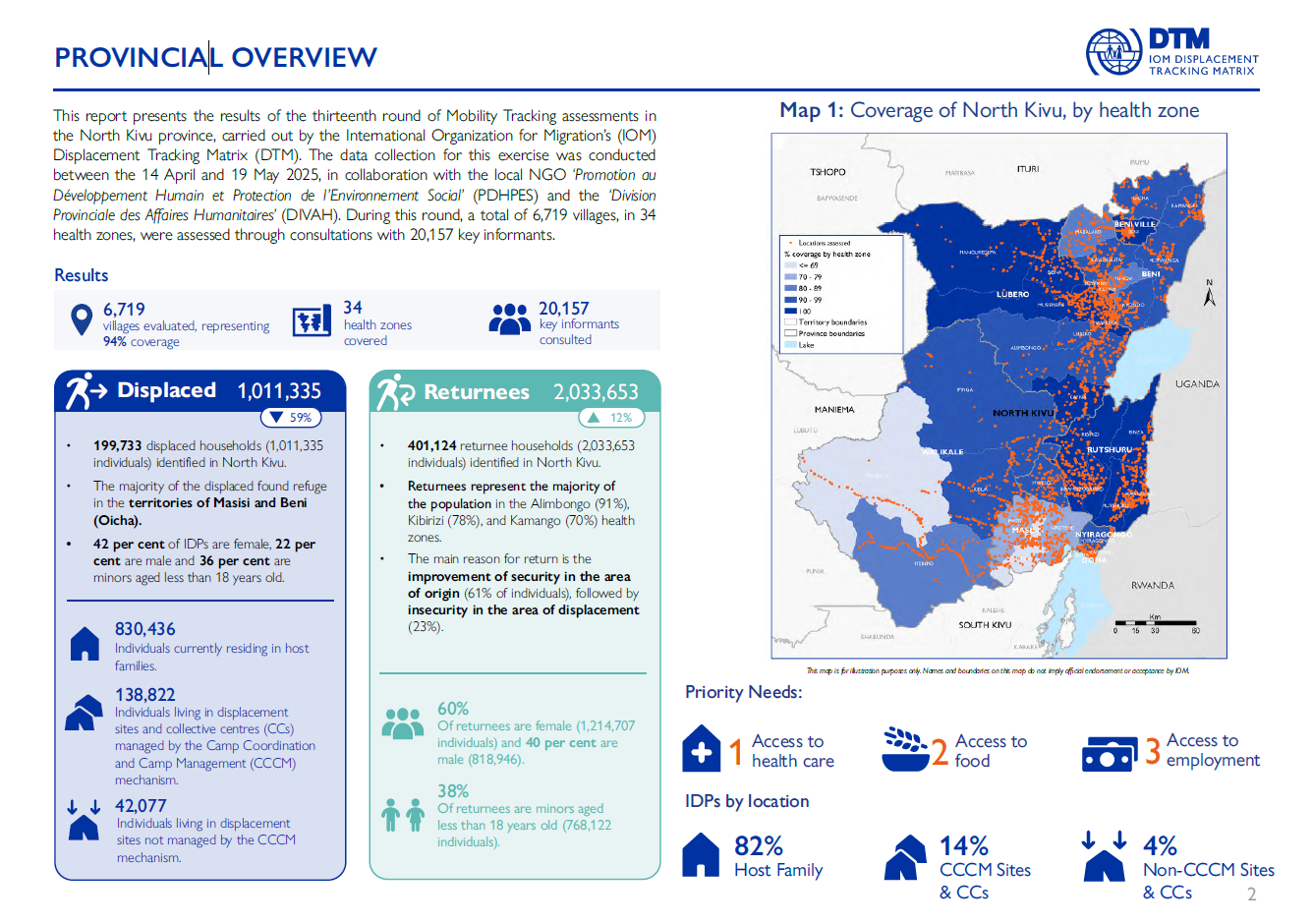
Page 1 Key Figures


#Page 1

#Assessment Date 

print('Top of Page')

try:
    assessment_Date_start = df_locations['m1855_meta_assessment_date'].min()
    assessment_Date_end = df_locations['m1855_meta_assessment_date'].max()
    print(f'Assessment date: {assessment_Date_start} to {assessment_Date_end}, unless otherwise specified.') 
except KeyError:
    print('not in date fotmat 1')

try:
    assessment_Date_start = df_locations['m2682_meta_date_auto'].min()
    assessment_Date_end = df_locations['m2682_meta_date_auto'].max()
    print(f'Assessment date: {assessment_Date_start} to {assessment_Date_end}, unless otherwise specified.') 
except KeyError:
    print('Not in date format 2')

#Num of Villages
number_of_Villages = df_locations['m0306_meta_adm4_label'].count()
print(f'Number of Villages {number_of_Villages}')
#Percentage Coverage
number_Villages_DPS = df_overview['Villages sur liste'].sum()    
coverage = number_of_Villages / number_Villages_DPS *100
print(f'Coverage: {coverage.round(0)}%')
#Num of ZS
number_of_ZS = df_locations['m0305_meta_adm3_pcode'].nunique()
print(f'Number of ZS: {number_of_ZS}')

#Num KIs
try:
    number_of_KIs = df_locations['m1729_loc_num_ki'].sum()
    print(f'Number of KIs {number_of_KIs}')
except KeyError:
    print('No KI code')

print("\n")

#Displacement Box
print('IDP Box')
#Total IDPs
total_IDPs_Host_Communities = df_grp_idp['x0010_grp_idp_ind'].sum()
total_IDPs_CCCM = df_cm['m0310_loc_num_idp_ind'].sum()
total_IDPs_Non_CCCM = df_ncm['m0310_loc_num_idp_ind'].sum()
total_IDPs = total_IDPs_Host_Communities + total_IDPs_CCCM + total_IDPs_Non_CCCM
total_IDPs = round(total_IDPs)
print(f'Total IDPs: {total_IDPs}')

#Total IDP change since previous round
total_IDP_Change = ((total_IDPs - previous_Total_IDPs)/previous_Total_IDPs) *100
print(f'Total IDP change {total_IDP_Change}%')

#Total IDP Households 
total_IDPs_Host_Communities_Households = df_grp_idp['x0009_grp_idp_hh'].sum()
total_IDPs_CCCM_Households = df_cm['m0309_loc_num_idp_hh'].sum()
total_IDPs_Non_CCCM_Households = df_ncm['m0309_loc_num_idp_hh'].sum()
total_IDP_Households = total_IDPs_Host_Communities_Households + total_IDPs_CCCM_Households + total_IDPs_Non_CCCM_Households
total_IDP_Households = round(total_IDP_Households)
print(f'Total IDP Households: {total_IDP_Households}')

#Majority of IDPs by Territory
majority_IDPs_admin_2_loc = df_grp_idp.groupby(['m0304_meta_adm2_label'])['x0010_grp_idp_ind'].sum()
majority_IDPs_admin_2_loc = majority_IDPs_admin_2_loc.reset_index()
majority_IDPs_admin_2_loc = majority_IDPs_admin_2_loc.rename(columns={'x0010_grp_idp_ind': 'm0310_loc_num_idp_ind'})
majority_IDPs_admin_2_cm = df_cm.groupby(['m0304_meta_adm2_label'])['m0310_loc_num_idp_ind'].sum()
majority_IDPs_admin_2_cm = majority_IDPs_admin_2_cm.reset_index()
majority_IDPs_admin_2_ncm = df_ncm.groupby(['m0304_meta_adm2_label'])['m0310_loc_num_idp_ind'].sum()
majority_IDPs_admin_2_ncm = majority_IDPs_admin_2_ncm.reset_index()
majority_IDPs_admin_2 = pd.concat([majority_IDPs_admin_2_loc, majority_IDPs_admin_2_cm, majority_IDPs_admin_2_ncm])
majority_IDPs_admin_2 = majority_IDPs_admin_2.groupby(['m0304_meta_adm2_label'])['m0310_loc_num_idp_ind'].sum() 
majority_IDPs_admin_2 = majority_IDPs_admin_2.sort_values(ascending=False)
print(f'The majority of IDPs found refuge in {majority_IDPs_admin_2.index[0].title()} and {majority_IDPs_admin_2.index[1].title()}')

#IDP Demographics

host_family_Males = df_locations['m2968_loc_num_men_idp'].sum()
host_family_Females = df_locations['m2969_loc_num_women_idp'].sum()
host_family_Children = df_locations['m2970_loc_num_children_idp'].sum()

male_IDPs = host_family_Males / total_IDPs_Host_Communities*100
female_IDPs = host_family_Females / total_IDPs_Host_Communities*100
children_IDPs = host_family_Children / total_IDPs_Host_Communities*100

subtraction = host_family_Children /2 
IDP_Men = host_family_Males - subtraction
IDP_Women = host_family_Females - subtraction
IDP_Men = IDP_Men / total_IDPs_Host_Communities*100
IDP_Women = IDP_Women / total_IDPs_Host_Communities*100

print(f'IDPs are {male_IDPs.round(1)}% male and {female_IDPs.round(1)}% female')
print(f'{IDP_Men.round(1)}% are men, {IDP_Women.round(1)}% are women, and {children_IDPs.round(1)}% are under 18 yo')

#IDP Individuals by Setting (Host Community, CCCM Camp or Non-CCCM Camp)
print(f'Total IDPs in Host Communities: {total_IDPs_Host_Communities}')
print(f'Total IDPs in CCCM Camps: {total_IDPs_CCCM.round(0)}')
print(f'Total IDPs in Non-CCCM Camps: {total_IDPs_Non_CCCM.round(0)}')
print("\n")

#Returnee Box 
print('Returnee Box')
#Total Returnees
total_RETs = df_grp_ret['x0034_grp_return_idp_ind'].sum()
print(f'Total Returnees: {total_RETs.round(0)}')

#Total RET change since previous round
total_RET_Change = ((total_RETs - previous_Total_RETs)/previous_Total_RETs) *100
print(f'Total RET change {total_RET_Change}%')

#Total RET Households 
total_RET_Households = df_grp_ret['x0033_grp_return_idp_hh'].sum()
print(f'Total RET Households: {total_RET_Households.round(0)}')

#Majority of Returnees by Health Zone in Host Communities
majority_RETs_admin_3 = df_grp_ret.groupby(['m0305_meta_adm3_label'])['x0034_grp_return_idp_ind'].sum()
majority_RETs_admin_3 = majority_RETs_admin_3.sort_values(ascending=False)
majority_RETs_admin_3 = majority_RETs_admin_3.reset_index()
total_Population_By_ZS = df_overview.groupby('Zone de sante')['Population 2023 (DPS)'].sum()
total_Population_By_ZS = total_Population_By_ZS.reset_index()
total_Population_By_ZS['Zone de sante'] = total_Population_By_ZS['Zone de sante'].str.upper()
majority_RETs_admin_3 = majority_RETs_admin_3.merge(total_Population_By_ZS, left_on='m0305_meta_adm3_label', right_on='Zone de sante')
majority_RETs_admin_3['Percentage'] = majority_RETs_admin_3['x0034_grp_return_idp_ind'] / majority_RETs_admin_3['Population 2023 (DPS)'] *100
majority_RETs_admin_3 = majority_RETs_admin_3.sort_values('Percentage', ascending=False).round(0)
majority_RETs_admin_3 = majority_RETs_admin_3.reset_index()
print(
    f'Returnees represent the majority of the population in the ' 
    f'{majority_RETs_admin_3['m0305_meta_adm3_label'][0].title()} {majority_RETs_admin_3['Percentage'][0]}%,' 
    f'{majority_RETs_admin_3['m0305_meta_adm3_label'][1].title()} {majority_RETs_admin_3['Percentage'][1]}% '
    f'and {majority_RETs_admin_3['m0305_meta_adm3_label'][2].title()} {majority_RETs_admin_3['Percentage'][2]}% health zones.'
    )

#RET Demographics

returnee_Males = df_locations['m2971_loc_num_men_return'].sum()
returnee_Females = df_locations['m2972_loc_num_women_return'].sum()
returnee_Children = df_locations['m2973_loc_num_children_return'].sum()

male_RETs = returnee_Males / total_RETs*100
female_RETs = returnee_Females / total_RETs*100
children_RETs = returnee_Children / total_RETs*100

subtraction = returnee_Children /2 
RET_Men = returnee_Males - subtraction
RET_Women = returnee_Females - subtraction
RET_Men = RET_Men / total_RETs*100
RET_Women = RET_Women / total_RETs*100

print(f'RETs are {male_RETs.round(1)}% male and {female_RETs.round(1)}% female')
print(f'There are {returnee_Males} male RETs, {returnee_Females} female RETs, and {returnee_Children} are children.')
print(f'{RET_Men.round(1)}% are men, {RET_Women.round(1)}% are women, and {children_RETs.round(1)}% are under 18 yo')
print("\n")

#Icon Row: Percentage IDPs by Shelter Type 
print('Icon Row: Percentage IDPs by Shelter Type ')
total_IDPs_Host_Communities_Percentage = total_IDPs_Host_Communities / total_IDPs *100
print(f'{total_IDPs_Host_Communities_Percentage.round(1)}% of IDPs in Host Communities')
total_IDPs_CCCM_Percentage = total_IDPs_CCCM / total_IDPs *100
print(f'{total_IDPs_CCCM_Percentage.round(1)}% of IDPs in CCCM Camps')
total_IDPs_Non_CCCM_Percentage = total_IDPs_Non_CCCM / total_IDPs *100
print(f'{total_IDPs_Non_CCCM_Percentage.round(1)}% of IDPs in Non-CCCM Camps')

Output of the Code

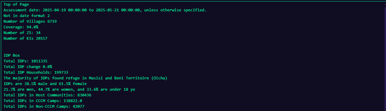
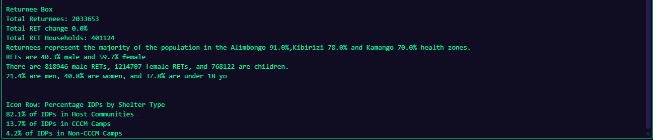
As you can see, the code’s output is relatively simple mathematics which give useful insights into the humanitarian situation in the east of the DRC. I’m a big fan of using the ‘try…except’ format on these data files because I can keep my workstream of analysis and validation running smoothly, even if I can’t quite get the depth of analysis I want all at once.

Analysis Page 2

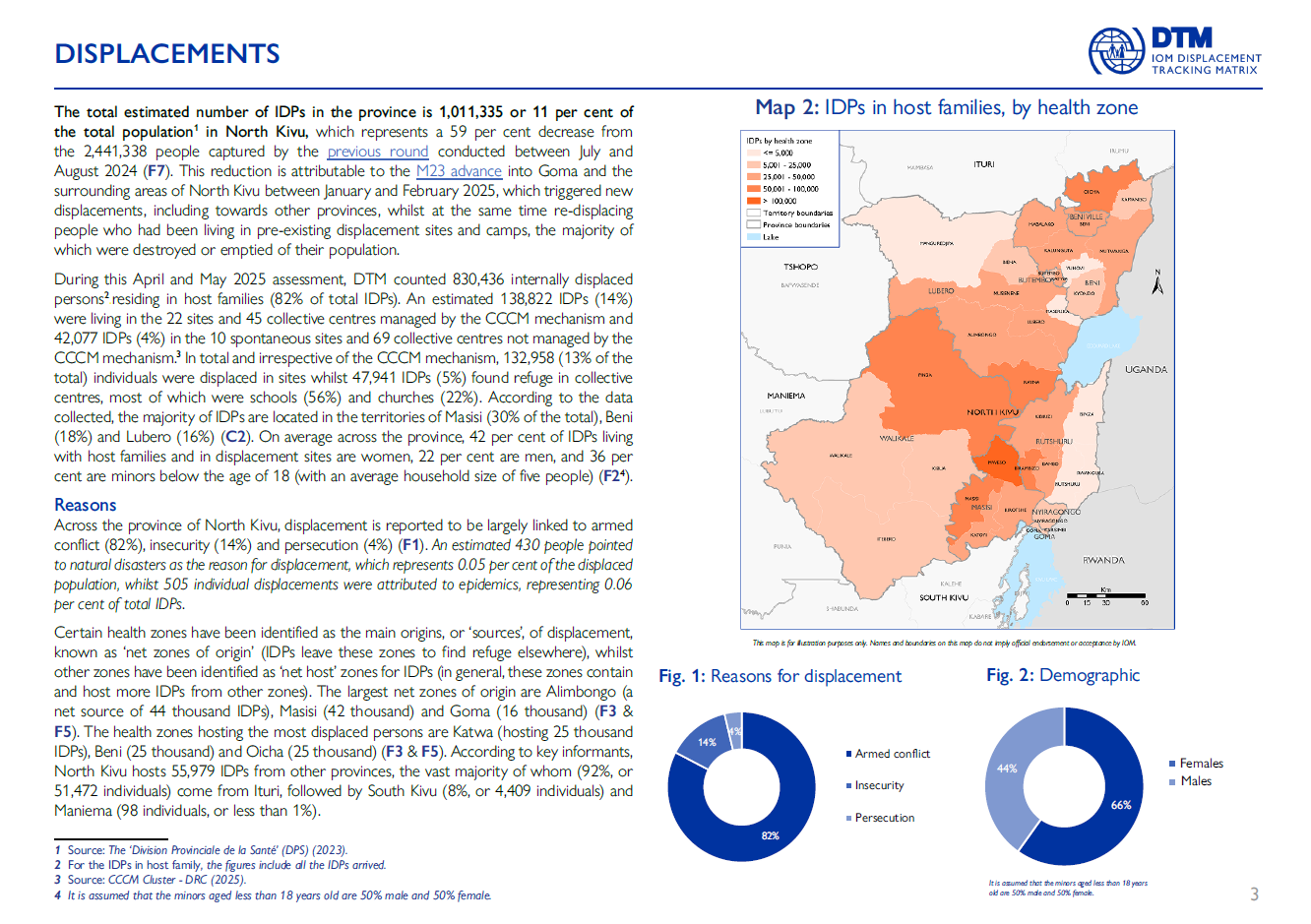
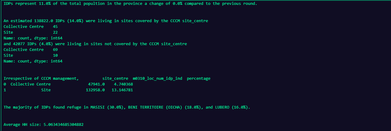
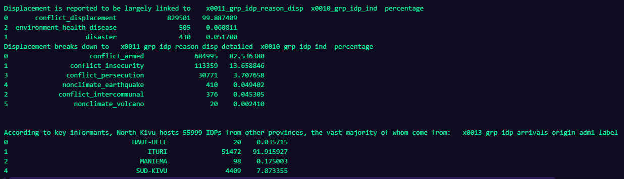
For page 2 and beyond, the calculations become a little more complicated conceptually but are still relatively simple, except for the ‘net source’ and ‘net host’ flow analysis at the bottom of the page. This is depicted in the second coding box.


#Page 2 

#Idps in province as % of total population and the change since the last reporting round

percent_Total_IDPs = total_IDPs / df_overview['Population 2023 (DPS)'] .sum() *100
number_CCCM_Sites = df_cm['site_centre'].value_counts() 
number_Non_CCCM_Sites = df_ncm['site_centre'].value_counts() 
print(
    f'IDPs represent {percent_Total_IDPs.round(0)}% of the total popultion in the province '
    f'a change of {total_IDP_Change}% compared to the previous round.'
    )
print("\n")

#Full Location Breakdown

print(
    f'An estimated {total_IDPs_CCCM} IDPs ({total_IDPs_CCCM_Percentage.round(0)}%) were living in sites covered by the CCCM ' 
    f'{number_CCCM_Sites} \n'
    f'and {total_IDPs_Non_CCCM} IDPs ({total_IDPs_Non_CCCM_Percentage.round(0)}%) were living in sites not covered by the CCCM ' 
    f'{number_Non_CCCM_Sites}'
)   
print("\n")

#IDPs in Sites and CCs irrespective of the CCCM 
  
sites_CC_CCCM = df_cm.groupby('site_centre')['m0310_loc_num_idp_ind'].sum()
sites_CC_CCCM = sites_CC_CCCM.reset_index()

sites_CC_Non_CCCM = df_ncm.groupby('site_centre')['m0310_loc_num_idp_ind'].sum()
sites_CC_Non_CCCM = sites_CC_Non_CCCM .reset_index()

sites_CC_Combined = pd.concat([sites_CC_CCCM,sites_CC_Non_CCCM],ignore_index=True)
sites_CC_Combined = sites_CC_Combined.groupby('site_centre')['m0310_loc_num_idp_ind'].sum()
sites_CC_Combined = sites_CC_Combined.reset_index()
sites_CC_Combined['percentage'] = sites_CC_Combined['m0310_loc_num_idp_ind'] / total_IDPs *100

print(f'Irrespective of CCCM management, {sites_CC_Combined}')
print("\n")

#More Detailed Majority of IDPs

majority_IDPs_admin_2 = majority_IDPs_admin_2.reset_index()
majority_IDPs_admin_2['percentage'] = majority_IDPs_admin_2['m0310_loc_num_idp_ind']/ total_IDPs *100
print(
    f'The majority of IDPs found refuge in {majority_IDPs_admin_2['m0304_meta_adm2_label'][0]} ' 
    f'({majority_IDPs_admin_2['percentage'][0].round()}%), {majority_IDPs_admin_2['m0304_meta_adm2_label'][1]} '
    f'({majority_IDPs_admin_2['percentage'][1].round()}%), and {majority_IDPs_admin_2['m0304_meta_adm2_label'][2]} '
    f'({majority_IDPs_admin_2['percentage'][2].round()}%).'
)

print("\n")

#Average Household Size

print(f'Average HH size: {total_IDPs/total_IDP_Households}')
print("\n")

#Reasons for Displacement Method 1 

displacement_Reasons_One = df_grp_idp.groupby('x0011_grp_idp_reason_disp')['x0010_grp_idp_ind'].sum()
displacement_Reasons_One = displacement_Reasons_One.reset_index()
displacement_Reasons_One['percentage'] = displacement_Reasons_One['x0010_grp_idp_ind'] / displacement_Reasons_One['x0010_grp_idp_ind'].sum() *100
displacement_Reasons_One = displacement_Reasons_One.sort_values(by='percentage', ascending=False)
print(
    f'Displacement is reported to be largely linked to{displacement_Reasons_One}'
)

#Reasons for Displacement Method 2

displacement_Reasons_Two = df_grp_idp.groupby('x0011_grp_idp_reason_disp_detailed')['x0010_grp_idp_ind'].sum()
displacement_Reasons_Two = displacement_Reasons_Two.reset_index()
displacement_Reasons_Two['percentage'] = displacement_Reasons_Two['x0010_grp_idp_ind'] / displacement_Reasons_Two['x0010_grp_idp_ind'].sum() *100
displacement_Reasons_Two = displacement_Reasons_Two.sort_values(by='percentage', ascending=False)
print(f'Displacement breaks down to {displacement_Reasons_Two}')

print("\n")

#Amount of IDPs the Province Hosts from Other Provinces

other_Provinces_IDPs = df_grp_idp.groupby('x0013_grp_idp_arrivals_origin_adm1_label')['x0010_grp_idp_ind'].sum()
other_Provinces_IDPs = other_Provinces_IDPs.reset_index()
other_Provinces_IDPs = other_Provinces_IDPs[other_Provinces_IDPs['x0013_grp_idp_arrivals_origin_adm1_label']!=ProvinceFR]
other_Provinces_IDPs_Total = other_Provinces_IDPs['x0010_grp_idp_ind'].sum()
other_Provinces_IDPs['percentage'] = other_Provinces_IDPs['x0010_grp_idp_ind'] / other_Provinces_IDPs_Total *100
print(
    f'According to key informants, {Province} hosts {other_Provinces_IDPs_Total} IDPs from other provinces, '
    f'the vast majority of whom come from: {other_Provinces_IDPs}'
)

The below code for the ‘Flow Analysis’ essentially comes down to organising the current location of IDPs against their places of origin (looking for where this matches or not) in order to determine two things: which health zones hosted the most IDPs and which were the sources of the most IDPs for this round (out of those in host communities only).


#Flow Analysis 

flow_ZS_IDPs = df_grp_idp.groupby(['m0305_meta_adm3_pcode', 'm0305_meta_adm3_label'])[['x0010_grp_idp_ind']].sum()
flow_ZS_IDPs = flow_ZS_IDPs.reset_index()

flow_ZS_Arrivals = df_grp_idp.groupby(['x0015_grp_idp_arrivals_origin_ZS','x0015_grp_idp_arrivals_origin_ZS_label'])[['x0010_grp_idp_ind']].sum()
flow_ZS_Arrivals = flow_ZS_Arrivals.reset_index()

flow_Analysis_ZS = flow_ZS_IDPs.merge(flow_ZS_Arrivals, left_on='m0305_meta_adm3_pcode', right_on='x0015_grp_idp_arrivals_origin_ZS', how='inner', suffixes=['_IDP','_Origin'])
flow_Analysis_ZS = flow_Analysis_ZS[['m0305_meta_adm3_label','x0010_grp_idp_ind_IDP','x0010_grp_idp_ind_Origin']]

flow_Analysis_ZS = flow_Analysis_ZS.rename(columns={'m0305_meta_adm3_label': 'Label', 'x0010_grp_idp_ind_IDP' : 'IDPs' , 'x0010_grp_idp_ind_Origin' : 'Origin'})

flow_Province = df_grp_idp.groupby('x0013_grp_idp_arrivals_origin_adm1_label')[['x0010_grp_idp_ind']].sum()
flow_Province = flow_Province.reset_index()
condition_1 = flow_Province['x0013_grp_idp_arrivals_origin_adm1_label']!= ProvinceFR
flow_Province = flow_Province[condition_1]

flow_Province = flow_Province.rename(columns={'x0013_grp_idp_arrivals_origin_adm1_label': 'Label', 'x0010_grp_idp_ind' : 'Origin'})

flow_Analysis = pd.concat([flow_Analysis_ZS, flow_Province], ignore_index=True)

flow_Analysis = flow_Analysis.fillna(0)

flow_Analysis['Flow/Flux'] = flow_Analysis['IDPs'] - flow_Analysis['Origin']
flow_Analysis = flow_Analysis.sort_values(by='Flow/Flux', ascending=False)

flow_Analysis_ZS['Flow/Flux'] = flow_Analysis_ZS['IDPs'] - flow_Analysis_ZS['Origin']
flow_Analysis_ZS = flow_Analysis_ZS.sort_values(by='Flow/Flux', ascending=False)

print(
    f'The largest net zones of origin/net hosts are {flow_Analysis_ZS['Label'].iloc[-1]} {flow_Analysis_ZS['Flow/Flux'].iloc[-1]} IDPs, '
    f'{flow_Analysis_ZS['Label'].iloc[-2]} {flow_Analysis_ZS['Flow/Flux'].iloc[-2]} IDPs, and '
    f'{flow_Analysis_ZS['Label'].iloc[-3]} {flow_Analysis_ZS['Flow/Flux'].iloc[-3]} IDPs.'
    )
print("\n")

print(
    f'The health zones hosting the most displaced persons/net sources are {flow_Analysis_ZS['Label'].iloc[0]} {flow_Analysis_ZS['Flow/Flux'].iloc[0]} IDPs, '
    f'{flow_Analysis_ZS['Label'].iloc[1]} {flow_Analysis_ZS['Flow/Flux'].iloc[1]} IDPs, and '
    f'{flow_Analysis_ZS['Label'].iloc[2]} {flow_Analysis_ZS['Flow/Flux'].iloc[2]} IDPs.'
    )

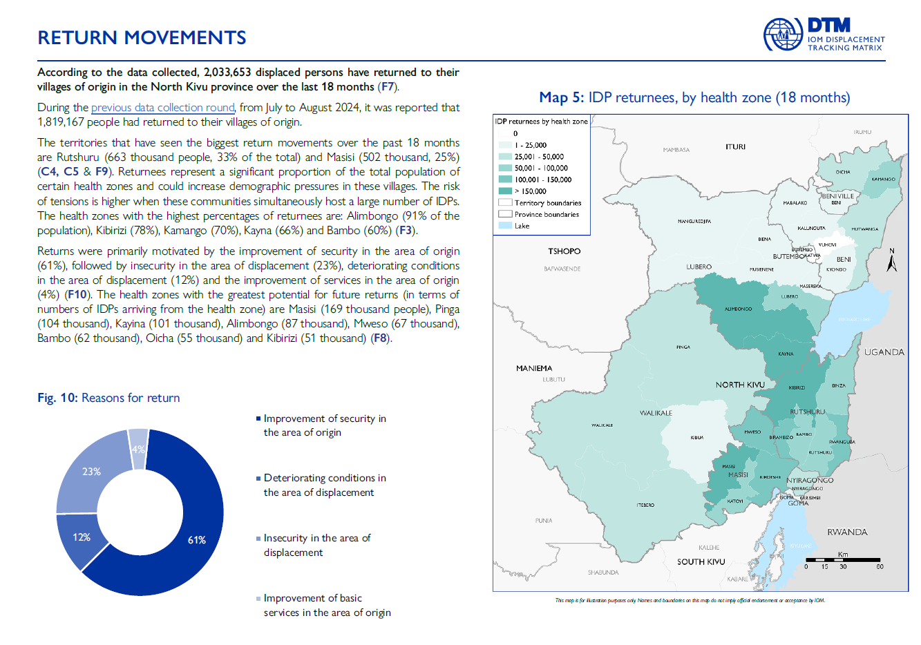
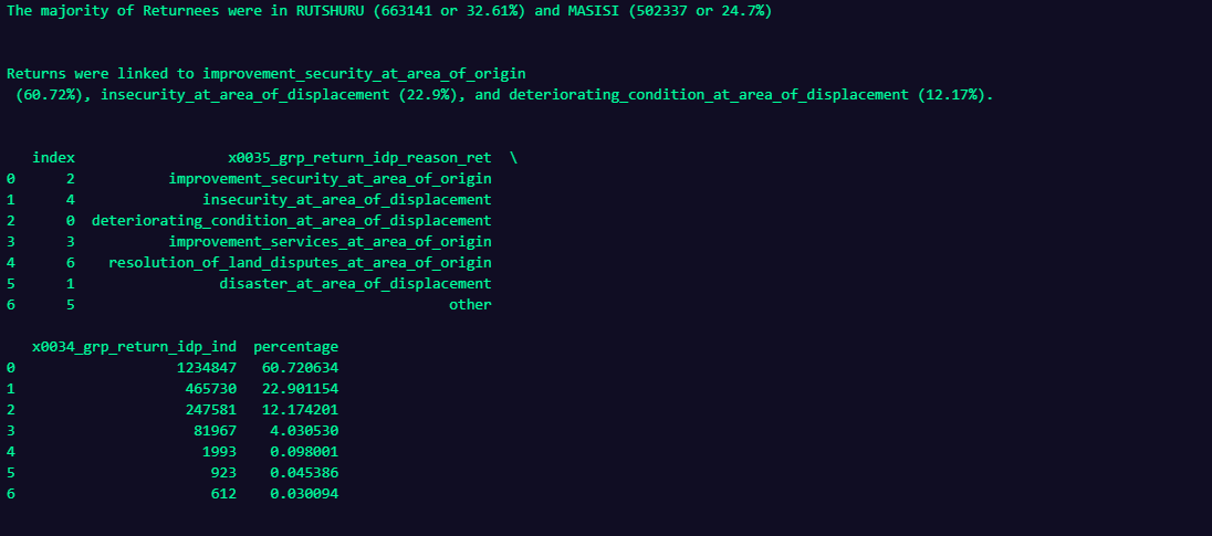
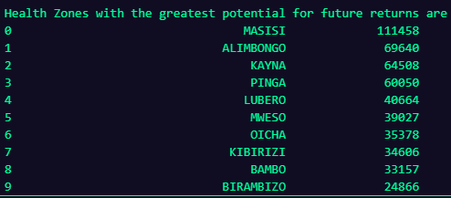
The next set of code is designed to give me the output from the Returnee page: the reasons for returning and the areas with the greatest potential for future returns.


#Returns Page 

#Majority of Returnees Admin 2

majority_RETs_admin_2 = df_grp_ret.groupby(['m0304_meta_adm2_label'])['x0034_grp_return_idp_ind'].sum() 
majority_RETs_admin_2 = majority_RETs_admin_2.reset_index()
majority_RETs_admin_2['percentage'] = majority_RETs_admin_2['x0034_grp_return_idp_ind'] / total_RETs *100
majority_RETs_admin_2 = majority_RETs_admin_2.sort_values(by='percentage', ascending=False)
majority_RETs_admin_2 = majority_RETs_admin_2.reset_index()
print(
    f'The majority of Returnees were in {majority_RETs_admin_2['m0304_meta_adm2_label'][0]} ({majority_RETs_admin_2['x0034_grp_return_idp_ind'][0]} '
    f'or {majority_RETs_admin_2['percentage'][0].round(2)}%) and {majority_RETs_admin_2['m0304_meta_adm2_label'][1]} '
    f'({majority_RETs_admin_2['x0034_grp_return_idp_ind'][1]} or {majority_RETs_admin_2['percentage'][1].round(2)}%)'
    )

print("\n")

#Reasons for Return
return_Reasons_One = df_grp_ret.groupby('x0035_grp_return_idp_reason_ret')['x0034_grp_return_idp_ind'].sum()
return_Reasons_One = return_Reasons_One.reset_index()
return_Reasons_One['percentage'] = return_Reasons_One['x0034_grp_return_idp_ind'] / return_Reasons_One['x0034_grp_return_idp_ind'].sum() *100
return_Reasons_One = return_Reasons_One.sort_values(by='percentage', ascending=False)
return_Reasons_One = return_Reasons_One.reset_index()
print(
    f'Returns were linked to {return_Reasons_One['x0035_grp_return_idp_reason_ret'][0]}\n ' 
    f'({return_Reasons_One['percentage'][0].round(2)}%), {return_Reasons_One['x0035_grp_return_idp_reason_ret'][1]} '
    f'({return_Reasons_One['percentage'][1].round(2)}%), and {return_Reasons_One['x0035_grp_return_idp_reason_ret'][2]} '
    f'({return_Reasons_One['percentage'][2].round(2)}%).'
)
print("\n")

print(return_Reasons_One)

print("\n")
#Health Zones with the Greatest Potential for Future Returns
future_Returns = df_grp_idp.groupby('x0015_grp_idp_arrivals_origin_ZS_label')['x0010_grp_idp_ind'].sum()
future_Returns = future_Returns.sort_values(ascending=False)
future_Returns = future_Returns.reset_index()
print(f'Health Zones with the greatest potential for future returns are {future_Returns.head(10)}')

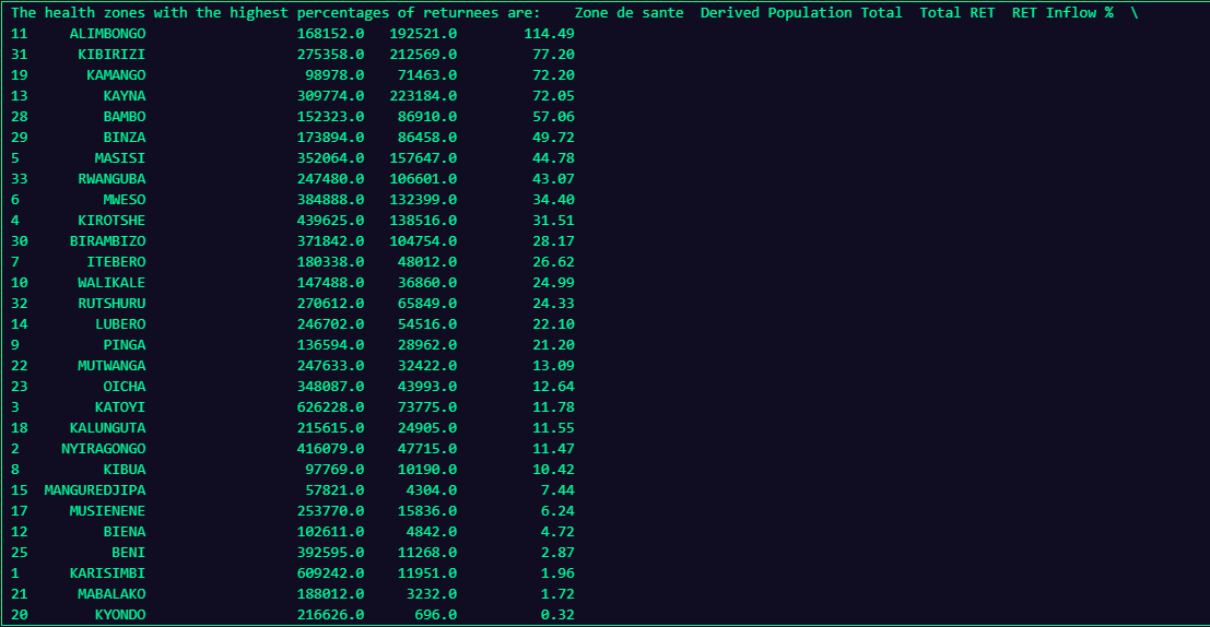
The next set of code is the calculation of the ‘Pressure Index’ which is essentially the Flow Analysis calculation from before, but with an estimated population total and the data from the displacement camps collected for the current round. The three columns in the output are the most important for the report, but there are several others, as depicted in the below code.


#Pressure Index

all_Flows_1 = df_overview.groupby('Zone de sante', as_index=False)['Population 2023 (DPS)'].sum()
all_Flows_1['Zone de sante'] = all_Flows_1['Zone de sante'].str.upper()
all_Flows_2 = df_overview.groupby('Pcode ZS', as_index=False)['Population 2023 (DPS)'].sum()
all_Flows = all_Flows_1.merge(all_Flows_2, left_on='Population 2023 (DPS)', right_on='Population 2023 (DPS)')

all_Flows=all_Flows.fillna(0)

influx_IDP = df_grp_idp[['m0305_meta_adm3_pcode','m0305_meta_adm3_label', 'x0010_grp_idp_ind','x0015_grp_idp_arrivals_origin_ZS']]
influx_Condition = df_grp_idp['m0305_meta_adm3_pcode'] != df_grp_idp['x0015_grp_idp_arrivals_origin_ZS']  
influx_IDP = influx_IDP[influx_Condition]
influx_IDP = influx_IDP.groupby(['m0305_meta_adm3_label'], as_index=False)['x0010_grp_idp_ind'].sum()

all_Flows = all_Flows.merge(influx_IDP, left_on='Zone de sante', right_on='m0305_meta_adm3_label', how='left')
all_Flows=all_Flows.fillna(0)

outflux_IDP = df_grp_idp[['m0305_meta_adm3_pcode','x0010_grp_idp_ind','x0015_grp_idp_arrivals_origin_ZS']]
outflux_Condition = df_grp_idp['m0305_meta_adm3_pcode'] != df_grp_idp['x0015_grp_idp_arrivals_origin_ZS'] # changed
outflux_IDP = outflux_IDP[outflux_Condition]
outflux_IDP = outflux_IDP.groupby('x0015_grp_idp_arrivals_origin_ZS', as_index=False)['x0010_grp_idp_ind'].sum()


all_Flows = all_Flows.merge(outflux_IDP, left_on='Pcode ZS', right_on='x0015_grp_idp_arrivals_origin_ZS', how='left')
all_Flows=all_Flows.fillna(0)

all_Flows = all_Flows[['m0305_meta_adm3_label','Pcode ZS','Zone de sante','Population 2023 (DPS)','x0010_grp_idp_ind_x','x0010_grp_idp_ind_y']]

all_Flows = all_Flows.rename(columns={
    'x0010_grp_idp_ind_x' : 'IDP Influx',
    'x0010_grp_idp_ind_y': 'IDPs Outflow'
})

all_Flows['Derived Population Total'] = all_Flows['Population 2023 (DPS)'] + all_Flows['IDP Influx'] - all_Flows['IDPs Outflow']

origin_IDP = df_grp_idp[['m0305_meta_adm3_pcode', 'x0010_grp_idp_ind','x0015_grp_idp_arrivals_origin_ZS']]
origin_Condition = df_grp_idp['m0305_meta_adm3_pcode'] == df_grp_idp['x0015_grp_idp_arrivals_origin_ZS']
origin_IDP = origin_IDP[origin_Condition]
origin_IDP = origin_IDP.groupby('m0305_meta_adm3_pcode', as_index=False)['x0010_grp_idp_ind'].sum()

all_Flows = all_Flows.merge(origin_IDP, left_on='Pcode ZS', right_on='m0305_meta_adm3_pcode', how='outer')
all_Flows = all_Flows.rename(columns={
    'x0010_grp_idp_ind' : 'IDP Origin'
})
all_Flows=all_Flows.fillna(0)

all_Flows = all_Flows[[
    'm0305_meta_adm3_label','Pcode ZS','Zone de sante','Population 2023 (DPS)','IDP Influx',
    'IDPs Outflow','Derived Population Total','IDP Origin']]

flows_CCCM = df_cm.groupby('m0305_meta_adm3_pcode', as_index=False)['m0310_loc_num_idp_ind'].sum()


all_Flows = all_Flows.merge(flows_CCCM, left_on='Pcode ZS', right_on='m0305_meta_adm3_pcode', how='outer')
all_Flows = all_Flows.rename(columns={
    'm0310_loc_num_idp_ind' : 'IDP CCCM'
})

all_Flows = all_Flows[[
    'm0305_meta_adm3_label','Pcode ZS','Zone de sante','Population 2023 (DPS)','IDP Influx','IDPs Outflow',
    'Derived Population Total','IDP Origin','IDP CCCM']]

flows_Non_CCCM = df_ncm.groupby('m0305_meta_adm3_pcode', as_index=False)['m0310_loc_num_idp_ind'].sum()


all_Flows = all_Flows.merge(flows_Non_CCCM, left_on='Pcode ZS', right_on='m0305_meta_adm3_pcode', how='outer')
all_Flows = all_Flows.rename(columns={
    'm0310_loc_num_idp_ind' : 'IDP Non-CCCM'
})

all_Flows = all_Flows.fillna(0)

all_Flows = all_Flows[[
    'm0305_meta_adm3_label','Pcode ZS','Zone de sante','Population 2023 (DPS)','IDP Influx','IDPs Outflow',
    'Derived Population Total','IDP Origin','IDP CCCM','IDP Non-CCCM']]

all_Flows['Total IDP'] = all_Flows['IDP Non-CCCM'] + all_Flows['IDP CCCM'] + all_Flows['IDP Origin']
all_Flows = all_Flows.fillna(0)

flows_RET = df_grp_ret.groupby('m0305_meta_adm3_pcode', as_index=False)['x0034_grp_return_idp_ind'].sum()


all_Flows = all_Flows.merge(flows_RET, left_on='Pcode ZS', right_on='m0305_meta_adm3_pcode',how='left') #how='outer'
all_Flows = all_Flows.rename(columns={
    'x0034_grp_return_idp_ind' : 'Total RET'
})
all_Flows = all_Flows.fillna(0)

all_Flows = all_Flows[[
    'm0305_meta_adm3_label','Pcode ZS','Zone de sante','Population 2023 (DPS)','IDP Influx','IDPs Outflow',
    'Derived Population Total','IDP Origin','IDP CCCM','IDP Non-CCCM','Total IDP',
    'Total RET']]

all_Flows['Not IDP/Returnee'] = all_Flows['Derived Population Total'] - all_Flows['IDP Influx'] - all_Flows['Total IDP'] - all_Flows['Total RET']

all_Flows['IDP Origin Same ZS'] = all_Flows['Total IDP'] / all_Flows['Derived Population Total'] *100
all_Flows['IDP Origin Same ZS'] = all_Flows['IDP Origin Same ZS'].round(2)

all_Flows['IDP Inflow %'] = all_Flows['IDP Influx'] / all_Flows['Derived Population Total'] *100
all_Flows['IDP Inflow %'] = all_Flows['IDP Inflow %'].round(2)

all_Flows['RET Inflow %'] = all_Flows['Total RET'] / all_Flows['Derived Population Total'] *100
all_Flows['RET Inflow %'] = all_Flows['RET Inflow %'].round(2)

all_Flows['Not IDP/RET %'] = all_Flows['Not IDP/Returnee'] / all_Flows['Derived Population Total'] *100
all_Flows['Not IDP/RET %'] = all_Flows['Not IDP/RET %'].round(2)

all_Flows['RET Inflow % 2'] = all_Flows['Total RET'] / all_Flows['Population 2023 (DPS)'] *100
all_Flows['RET Inflow % 2'] = all_Flows['RET Inflow % 2'].round(2)

all_Flows = all_Flows.sort_values(by='RET Inflow %', ascending=False)

print(f'The health zones with the highest percentages of returnees are: {all_Flows[['Zone de sante', 'Derived Population Total', 'Total RET', 'RET Inflow %', 'RET Inflow % 2']]}')

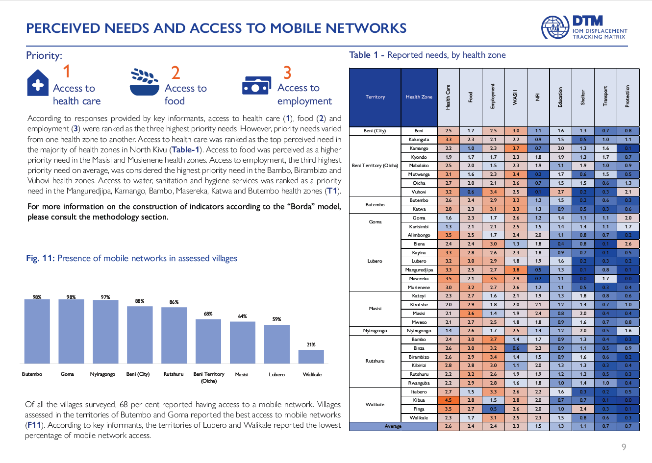
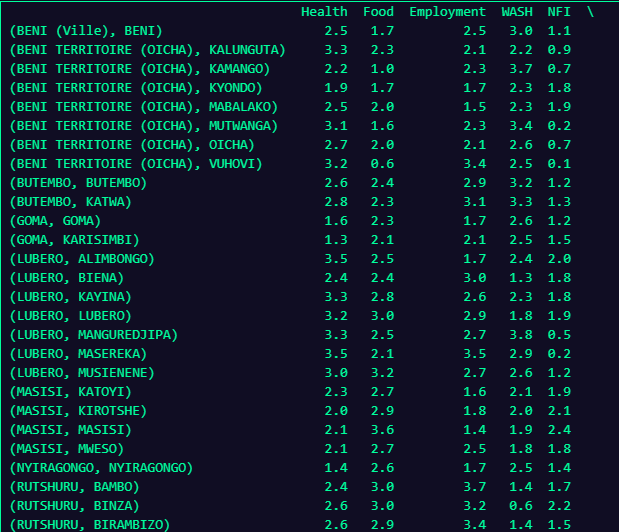
The final three parts of code consist of the following: a simple calculation for the percentage of mobile coverage and a two-part set of code which builds Table 1 in the below image (the code output shown is only partial). The table is a really great way of visualising the priority needs of different health zones across the province and also informs the overall or ‘Average’ three priority needs across the sample of the province.


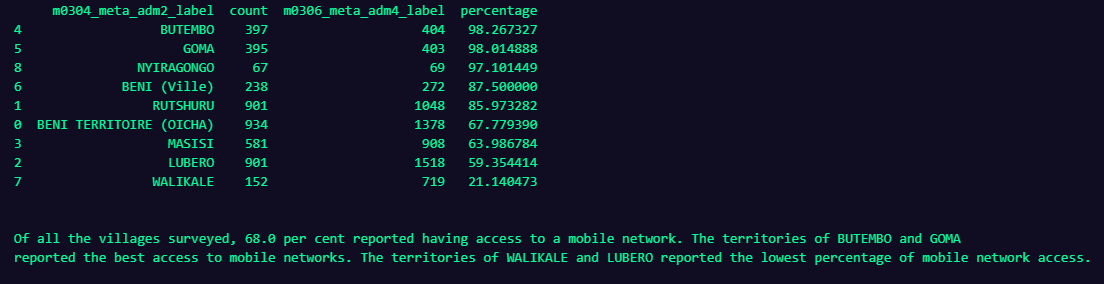
#Mobile Service Coverage
mobile_Cov = df_locations[['m0304_meta_adm2_label','s1784_loc_mobile_access']].value_counts()
mobile_Cov = mobile_Cov.reset_index()
mob_condition = mobile_Cov['s1784_loc_mobile_access'] == 'yes'
mobile_Cov = mobile_Cov[mob_condition]
mobile_Cov = mobile_Cov[['m0304_meta_adm2_label','count']]

villages_By_Territory = df_locations.groupby('m0304_meta_adm2_label')['m0306_meta_adm4_label'].count()
villages_By_Territory = villages_By_Territory.reset_index()

total_Cov = mobile_Cov['count'].sum()
total_Cov = total_Cov / number_of_Villages *100

mobile_Cov_Admin_2 = mobile_Cov.merge(villages_By_Territory, on='m0304_meta_adm2_label')
mobile_Cov_Admin_2['percentage'] = mobile_Cov_Admin_2['count'] / mobile_Cov_Admin_2['m0306_meta_adm4_label'] *100
mobile_Cov_Admin_2 = mobile_Cov_Admin_2.sort_values(by='percentage', ascending=False)
print(mobile_Cov_Admin_2)

print("\n")

print(
f'Of all the villages surveyed, {total_Cov.round(0)} per cent reported having access to a mobile network. ' 
f'The territories of {mobile_Cov_Admin_2['m0304_meta_adm2_label'].iloc[0]} and {mobile_Cov_Admin_2['m0304_meta_adm2_label'].iloc[1]} \n'
f'reported the best access to mobile networks. The territories of {mobile_Cov_Admin_2['m0304_meta_adm2_label'].iloc[-1]} '
f'and {mobile_Cov_Admin_2['m0304_meta_adm2_label'].iloc[-2]} reported the lowest percentage of mobile network access.'
)


#Priority Needs Part 1

df_loc_borda = df_locations[['m0304_meta_adm2_label', 'm0305_meta_adm3_label', 'm1560_loc_first_important_need',
'm1561_loc_second_important_need','m1562_loc_third_important_need', 'm1563_loc_fourth_important_need', 'm1564_loc_fifth_important_need']]
# List of Needs: 'health','nfi','wash','education','food', 'employment', 'transport', 'protection', 'shelter', 'other

# Health
df_loc_borda['Health'] = np.where(df_loc_borda['m1560_loc_first_important_need'] == 'health', 5,
np.where(df_loc_borda['m1561_loc_second_important_need'] == 'health', 4,
np.where(df_loc_borda['m1562_loc_third_important_need'] == 'health', 3,
np.where(df_loc_borda['m1563_loc_fourth_important_need'] == 'health', 2,
np.where(df_loc_borda['m1564_loc_fifth_important_need'] == 'health', 1,0
)))))

# NFI
df_loc_borda['NFI'] = np.where(df_loc_borda['m1560_loc_first_important_need'] == 'nfi', 5,
np.where(df_loc_borda['m1561_loc_second_important_need'] == 'nfi', 4,
np.where(df_loc_borda['m1562_loc_third_important_need'] == 'nfi', 3,
np.where(df_loc_borda['m1563_loc_fourth_important_need'] == 'nfi', 2,
np.where(df_loc_borda['m1564_loc_fifth_important_need'] == 'nfi', 1,0
)))))

# WASH
df_loc_borda['Education'] = np.where(df_loc_borda['m1560_loc_first_important_need'] == 'education', 5,
np.where(df_loc_borda['m1561_loc_second_important_need'] == 'education', 4,
np.where(df_loc_borda['m1562_loc_third_important_need'] == 'education', 3,
np.where(df_loc_borda['m1563_loc_fourth_important_need'] == 'education', 2,
np.where(df_loc_borda['m1564_loc_fifth_important_need'] == 'education', 1,0
)))))

df_loc_borda['WASH'] = np.where(df_loc_borda['m1560_loc_first_important_need'] == 'wash', 5,
np.where(df_loc_borda['m1561_loc_second_important_need'] == 'wash', 4,
np.where(df_loc_borda['m1562_loc_third_important_need'] == 'wash', 3,
np.where(df_loc_borda['m1563_loc_fourth_important_need'] == 'wash', 2,
np.where(df_loc_borda['m1564_loc_fifth_important_need'] == 'wash', 1,0
)))))

df_loc_borda['Food'] = np.where(df_loc_borda['m1560_loc_first_important_need'] == 'food', 5,
np.where(df_loc_borda['m1561_loc_second_important_need'] == 'food', 4,
np.where(df_loc_borda['m1562_loc_third_important_need'] == 'food', 3,
np.where(df_loc_borda['m1563_loc_fourth_important_need'] == 'food', 2,
np.where(df_loc_borda['m1564_loc_fifth_important_need'] == 'food', 1,0
)))))

df_loc_borda['Employment'] = np.where(df_loc_borda['m1560_loc_first_important_need'] == 'employment', 5,
np.where(df_loc_borda['m1561_loc_second_important_need'] == 'employment', 4,
np.where(df_loc_borda['m1562_loc_third_important_need'] == 'employment', 3,
np.where(df_loc_borda['m1563_loc_fourth_important_need'] == 'employment', 2,
np.where(df_loc_borda['m1564_loc_fifth_important_need'] == 'employment', 1,0
)))))

df_loc_borda['Protection'] = np.where(df_loc_borda['m1560_loc_first_important_need'] == 'protection', 5,
np.where(df_loc_borda['m1561_loc_second_important_need'] == 'protection', 4,
np.where(df_loc_borda['m1562_loc_third_important_need'] == 'protection', 3,
np.where(df_loc_borda['m1563_loc_fourth_important_need'] == 'protection', 2,
np.where(df_loc_borda['m1564_loc_fifth_important_need'] == 'protection', 1,0
)))))

df_loc_borda['Transport'] = np.where(df_loc_borda['m1560_loc_first_important_need'] == 'transport', 5,
np.where(df_loc_borda['m1561_loc_second_important_need'] == 'transport', 4,
np.where(df_loc_borda['m1562_loc_third_important_need'] == 'transport', 3,
np.where(df_loc_borda['m1563_loc_fourth_important_need'] == 'transport', 2,
np.where(df_loc_borda['m1564_loc_fifth_important_need'] == 'transport', 1,0
)))))

df_loc_borda['Shelter'] = np.where(df_loc_borda['m1560_loc_first_important_need'] == 'shelter', 5,
np.where(df_loc_borda['m1561_loc_second_important_need'] == 'shelter', 4,
np.where(df_loc_borda['m1562_loc_third_important_need'] == 'shelter', 3,
np.where(df_loc_borda['m1563_loc_fourth_important_need'] == 'shelter', 2,
np.where(df_loc_borda['m1564_loc_fifth_important_need'] == 'shelter', 1,0
)))))

df_loc_borda['Other'] = np.where(df_loc_borda['m1560_loc_first_important_need'] == 'other', 5,
np.where(df_loc_borda['m1561_loc_second_important_need'] == 'other', 4,
np.where(df_loc_borda['m1562_loc_third_important_need'] == 'other', 3,
np.where(df_loc_borda['m1563_loc_fourth_important_need'] == 'other', 2,
np.where(df_loc_borda['m1564_loc_fifth_important_need'] == 'other', 1,0
)))))


#Priority Needs Part 2

borda_Count = df_loc_borda.groupby(['m0304_meta_adm2_label', 'm0305_meta_adm3_label'])[['Health','NFI','WASH','Education','Food', 'Employment', 'Transport', 'Protection', 'Shelter', 'Other']].mean()
borda_Count = borda_Count.reset_index()
borda_Count = borda_Count.set_index(['m0304_meta_adm2_label', 'm0305_meta_adm3_label'])

borda_Total = df_loc_borda[['m0304_meta_adm2_label', 'm0305_meta_adm3_label','Health','NFI','WASH','Education','Food', 'Employment', 'Transport', 'Protection', 'Shelter', 'Other']]
borda_Total = borda_Total.set_index(['m0304_meta_adm2_label', 'm0305_meta_adm3_label'])
borda_Total = borda_Total.mean()
borda_Count.loc['Grand Total'] = borda_Total

average_Col = borda_Count[['Health','NFI','WASH','Education','Food', 'Employment', 'Transport', 'Protection', 'Shelter']].sum(axis=1)
average_Col = 15 / average_Col

borda_Count_2 = borda_Count[['Health','NFI','WASH','Education','Food', 'Employment', 'Transport', 'Protection', 'Shelter']]
borda_Final = borda_Count_2.multiply(average_Col, axis=0)

ranked = borda_Final.loc['Grand Total']
ranked = ranked.sort_values(ascending=False).index
ranked = borda_Final[ranked]

print(ranked.round(1))

End of Part 1

There you have it, some useful code for some simple and insightful analysis.